Lab 5 - Electromagnetic Transients in Power Systems
ECE433 - Power Systems Stability and Transients
Electrical and Computer Engineering - University of Alberta

figure 1: Power Station
1 Introduction
The analysis and simulation of electromagnetic transients has become a fundamental methodology for understanding the performance of power systems. It is an important tool in designing and determining the component ratings that make up the system. It is also used to explain equipment failures as well as testing protection devices. In this lab a popular tool for Power Systems EMT (Electromagnetic Transient) simulations called PSCAD will be used to demonstrate through simulation a few different scenarios of electromagnetic transients in power systems.
1.1 Summary
Task 1 - Run a Sample Case
Learn the basics of the software package PSCAD by opening and running a simple example case that demonstrates a transient that is very easy to understand. This case examines the transient that happens when a bus is shorted by a fault, where that shorted bus is connected to an AC supply through a transmission line which is modeled with a single inductor.
Task 2 - Build a New Case - Capacitor Energization
Continue to learn the PSCAD environment by building a new circuit and performing multiple simulation scenarios on it. The circuit demonstrates several transient scenarios that can occur when a capacitor gets connected to the system.
Task 3 - Back-to-back Capacitor Energization
Expanding on the last task, a second capacitor is added in parallel to the existing system and the transient that occurs when the new capacitor is connected is examined.
1.2 Required Software
PSCAD (Power Systems CAD) is a powerful and flexible graphical user interface to the world- renowned, EMTDC solution engine. PSCAD enables the user to schematically construct a circuit, run a simulation, analyze the results, and manage the data in a completely integrated, graphical environment. Online plotting functions, controls and meters are also included, so that the user can alter system parameters during a simulation run, and view the results directly.
- Recommended version - PSCAD X4 (v4.6) - PSCAD Website
figure 2. PSCAD - Visual Simulation for Power Systems
PSCAD comes complete with a library of pre-programmed and tested models, ranging from simple passive elements and control functions, to more complex models, such as electric machines, FACTS devices, transmission lines and cables. If a particular model does not exist, PSCAD provides the flexibility of building custom models, either by assembling those graphically using existing models, or by utilizing an intuitively designed Design Editor.
The following are some common models found in systems studied using PSCAD:
Resistors, inductors, capacitors
Mutually coupled windings, such as transformers
Switches and breakers
Protection and relaying
Diodes, thyristors and GTOs
Analog and digital control functions
AC and DC machines, exciters, governors,
Frequency dependent transmission lines and cables
Current and voltage sources stabilizers and inertial models
Meters and measuring functions
Generic DC and AC controls
HVDC, SVC, and other FACTS controllers
Wind source, turbines and governors
2 Pre-lab
Please complete the following before attending your scheduled lab session.
2.1 Pre-lab Tasks
Make sure you know where and when to come to the lab by looking at the lab schedule that is available on eClass.
Familiarize yourself with the lab procedures and requirements by reading through the lab manual.
Complete the questions from the ECE433 - Lab 5 - Prelab Questions template. The same questions are shown below.
Have the ECE433 - Lab 5 – Sign-off sheet printed off before coming to the lab.
Note that there is a ECE433 - Lab 5 - Postlab template for you to complete and submit. You will need to collect the required graphs to include in your lab report as well as answer the postlab questions that are both shown in the template as well as inline in the lab manual.
2.2 Pre-lab Questions
What are electromagnetic transients, and how are they different from electromechanical transients?
Why is the study of electromagnetic transients important in power systems design?
What is transient recovery voltage (TRV)?
Why are there electromagnetic transients when a capacitor is connected to a system?
How many resonant frequencies are there when a second capacitor branch is added in parallel to a operating system that already has an existing capacitor (ie. A back-to-back capacitor energization)?
How does the simulation time step affect simulation results?
3 Lab Procedure
3.1 Run a Sample Case
In order to introduce PSCAD, a sample case file will be used to demonstrate how to run and examine a simple simulation. This example file contains the simulation of a non-ideal single phase AC supply that is connected to a breaker that gets shorted to ground once activated through an inductor. The inductor is used as a simple model of a transmission line and the breaker is modeling a line to ground fault that occurs after a set time period during the simulation.
- Download the .zip file from below which contains the Lab 5 Sample
case that will be used for the first part of this lab. Extract it
somewhere you can find in your user space like your Desktop. The
extracted .zip file contains a single .pscx file titled
Lab_5_Sample_case.pscx.
Sample Case Download
- Open the extracted file in PSCAD by either double clicking on the
file or first launching PSCAD and using the menus to open the project.
Once open use the
Runbutton on the toolbar to simulate the case.
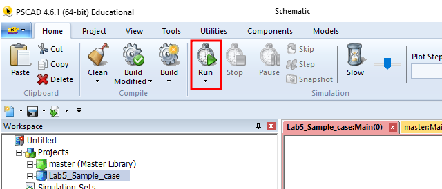
figure 3. Run button.
- It may take a few moments for the simulation to complete but once it does you should see something like the following displayed in the PSCAD main window.
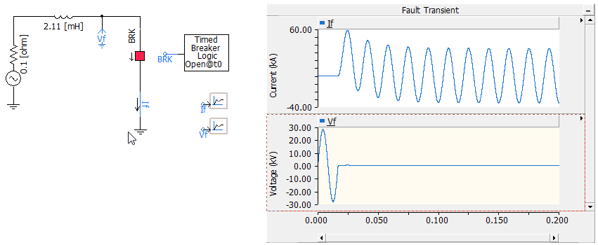
figure 4. Example case simulation result.
Take a few moments to play around and explore the interface. You may want become familiar with the following.
- The Zoom controls for the waveforms.
- Double clicking and right clicking on the different components to see what comes up.
- The menus of the toolbar ribbon, how they are organized and where things can be found.
During the lab you will be asked to save waveforms to include with your postlab report. The simplest way to do this with PSCAD is to do the following. Right click on either the graph itself to copy only a single graph, or right click on the title bar of the graph pane to copy all graphs in that pane. In the menu that comes up select
Copy as Meta-Fileto place the waveforms in your clipboard. You can then paste the waveform as an image in other software like MS Word. For all graphs, use the entire simulation time as the duration unless otherwise specified.
3.1.1 Postlab Graphs
G1. Use the fault transient simulation above to generate 2 sets of
currents and voltage waveforms. For the first set of waveforms use the
default value of 0.01667 s for the
Time of First Breaker Operation for the
Timed Breaker Logic Open@t0. For the second set of
waveforms change the time to 0.02084 s and see how the waveforms change.
Include these waveforms in your lab report.
3.1.2 Postlab Questions
Q1. Looking at only the first case with a closing time of 0.01667 s, explain what is happening in the simulation before and after the fault.
Q2. Explain why a breaker with a different closing time in the simulation would cause the resulting waveform to look different. Are there any potential problems because of this?
3.2 Build a New Case - Capacitor Energization
For the second task we are going to create a new simulation case from scratch to explore the transients that occur during the energization of a capacitor.
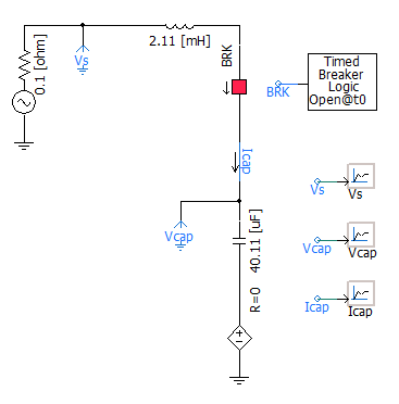
figure 5. Capacitor energization schematic.
Create a new case for this task (from File menu, select New and click on Case).
The components needed to create the circuit can be located in the following 2 locations.
- The
Master Libraryof PSCAD. To have access to this library double click on master (Master Library) icon in the workspace. Components can be copied and pasted to the main work window.
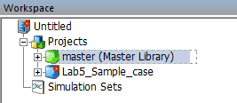
figure 6. Master library.
The ribbon tabs:
ComponentsandModels.- The
Componentsribbon contains the most commonly used items that make up your schematic drawing. It is mainly included for ease of use as most items also exist somewhere else in the interface. It Includes things like the passives, wires, meters, graphs and controls. TheComponentsribbon is shown below.
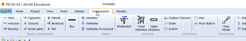
figure 7. Components ribbon tab.
- The
Modelsribbon contains all of the simulation models that are included with PSCAD and is used to access the, less used, more complex models that make up your schematic drawing. They are arranged in groups by the models function. TheModelsribbon is shown below.
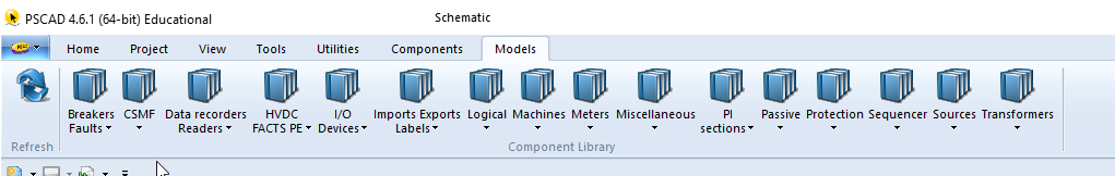
figure 8. Models ribbon tab.
- The
The procedure to create the circuit is explained in detail in the following sections. You may add components to your circuit in whichever way you wish however the second method (using ribbons) will be shown throughout the remainder of the lab manual.
- The
3.2.1 Insert Inductor
Add an inductor to model a simple transmission line by following the steps below.
- From the
Componentsribbon, under theSimple Componentsgroup insert anInductorinto your schematic.
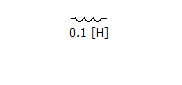
figure 9. Add an inductor.
Double click on the inductor or right click and select
Edit Parameters...to open up the inductor parameter control window.Set the inductance to
2.11 mH.
- From the
3.2.2 Insert Voltage Source
Add a AC voltage source to model a constant AC voltage bus to the system by following the steps below.
- From the
Modelsribbon, underSourcesinsert a[source_1] Single Phase Voltage Source Model 2into your schematic as shown below. Note that you can rotate a schematic element usingCtrl+Ror by right clicking on the component and going toOrientationin the context menu.
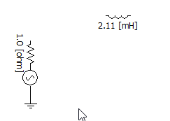
figure 10. Add a voltage source.
- Open the parameter control window and note that it has multiple sections that can be selected used the dropdown box at the top.
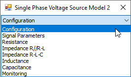
figure 11. Voltage source parameter sections.
- Set the Configuration, Signal Parameters, and Resistance parameters as shown in the figures below.
- From the
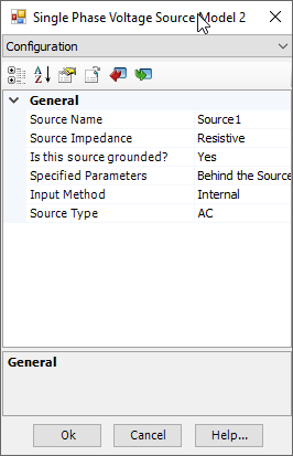
figure 12. Configuration (Voltage source).
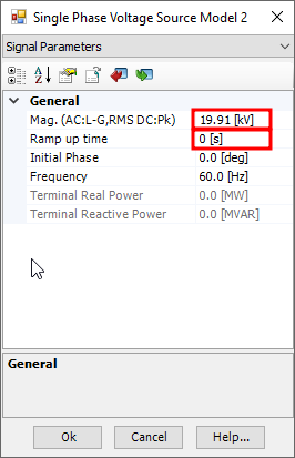
figure 13. Signal Parameters (Voltage source).
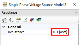
figure 14. Resistance (Voltage source).
3.2.3 Insert Breaker
Add a breaker with its control that initially has the breaker open and closes the breaker to connect the attached capacitor branch to the system after a certain time has elapsed. Follow the steps below to add this to the schematic.
From the
Modelsribbon, underBreakers Faultsadd both a[breaker1] Single Phase Breakerand a[tbreakn] Timed Breaker Logicto your schematic as shown below.From the
Componentsribbon, under theDataribbon group, insert aData labelnext to the Timed Breaker Logic port. TheData Signal Nameneeds to match theBreaker Namein order for the two components to be connected. These names can be edited in each of the components parameter control windows.
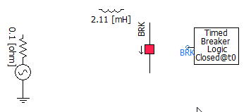
figure 15. Add a breaker and its control.
- Open the parameter control window for both the Breaker and the Timed Breaker Logic to edit their parameters as shown below.
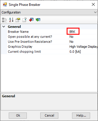
figure 16. Configuration (Breaker).
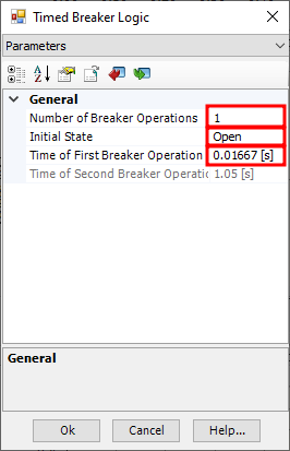
figure 17. Parameters (Timed Breaker Logic).
3.2.4 Insert Capacitor
Add a capacitor to the circuit as this is the type of load we want to add to the circuit to determine its transient behavior. In order to simulate a capacitor that is pre-charged we will also add a DC voltage source in series with the capacitor. Follow the steps below to add these 2 components to the schematic.
From the
Componentsribbon, under theSimple Componentsgroup insert anCapacitorinto your schematic as shown below.From the
Modelsribbon, underSourcesinsert another[source_1] Single Phase Voltage Source Model 2into your schematic as shown below.
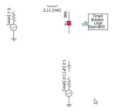
figure 18. Add capacitor and its pre-charge voltage source.
Open the Capacitors parameter control window and set the Capacitance to
40.11 uFFor the new voltage source configure its parameters as follows.
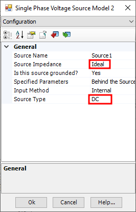
figure 19. Configuration (Pre-charge source).
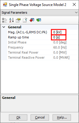
figure 20. Signal Parameters (Pre-charge source).
3.2.5 Insert Meters
In order select the quantities that need to be measured, meters need to be inserted in the schematic. Follow the steps below to insert the desired meters.
From the
Componentsribbon, under theMetersgroup, insert anAmmeterand the twoVoltmeter to Groundas shown below. Rename each meter as listed below by opening the parameter control window and changing itsSignal Nameto the appropriate one.- Vs
- Vcap
- Icap
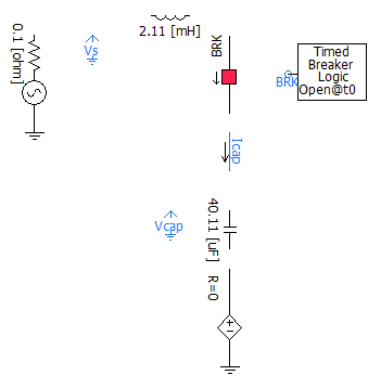
figure 21. Add 2 voltmeters and an ammeter.
3.2.6 Wire Components
To complete the schematic the components need to be connected together. To do this we use a wire tool. Follow the steps below to complete the wiring of the schematic.
- Activate wiring mode by clicking on the
Wire Modebutton, as shown below, on either theHomeorComponentsribbon.

figure 22. Wire tool.
- Left click were you want the wire to start. If you left click again an anchor point will be created for the wire. Right click where you want the wire to end. Note the excerpt from the PSCAD help files on what makes a valid connection below.
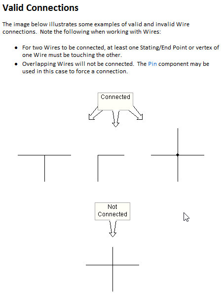
figure 23. Wiring connections.
- Complete all the wiring until your schematic looks like the following.
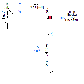
figure 24. Complete wiring with the wire tool.
- After completing the wiring you can either hit
ESCor click on theWire Modebutton again to deactive the wiring tool.
- Activate wiring mode by clicking on the
3.2.7 Simulation Settings
The simulation settings are important to setup properly so the desired information can be viewed efficiently. The idea is to set the
Duration of Runto the minimum required in order to see all of the desired events and their induced transient response. TheSolution Time Stepshould be set to a sufficiently low value that allows you capture the required frequency information without being to small that the simulation takes too long to simulate or creates excessively large amounts of data.- In the
Projectribbon, set the simulation time parameters as shown below.
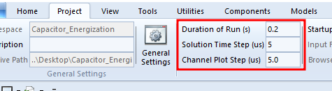
figure 25. Simulation time settings
- At this point you can try running the simulation by going to the
Homeribbon and clicking on the theRunbutton.
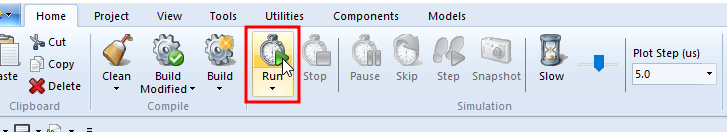
figure 26. Run button
- Look in the
Build Messagesdialog window located in the lower right of the PSCAD application. There should be some messages that pop up as the simulation proceeds. If there are any errors or warnings that pop up try and fix them before moving on to the next section.
- In the
3.2.8 Display Waveforms
As you may have noticed, no results are currently shown after simulation. Output channels and graph panes are needed to view the results. Here are the steps to add the required output channels and graph panes.
Add output channels.
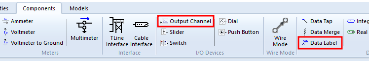
figure 27. Add a output channel and data label.
From the
Componentsribbon select theOutput Channeland place 3 of them in your schematic. One for each signal that you would like to measure. Name the 3Output Channelsyou just placed by going into their parameter controls window and changing thetitleentry to the following.- Supply Voltage
- Capacitor Voltage
- Capacitor Current
Again from the
Componentsribbon select theData Labeland place one next to each of the output channels you just created in the previous step. Go into the parameter control window for eachData Labeland change the signal name to the following making sure it coordinates with both the output channels name and the corresponding meter’s name.- Vs
- Vcap
- Icap
If required use a wire to connect the
Output Channelto the correspondingData Label.It doesn’t really matter where in the schematic theses output channels are placed but they should look something like the following when completed.
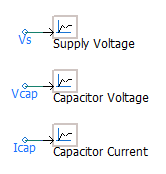
figure 28. Example of output channels setup.
Add a graph pane with overlays and connect them to the output channel data.
From the
Componentsribbon, under theGraphsgroup, select theGraph Paneand place it somewhere in your schematic where it is not on top of the stuff that you have already drawn there.On the top title bar of the newly inserted
Graph Pane, right click and selectAdd Overlay Graph (Analog)to insert a blank graph grid. Do this a total of 3 times to create 3 separate graphs so we can plot our 3 measurements on them.
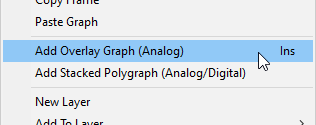
figure 29. Add overlay graphs.
Select the
Graph Paneon the top title bar so the resizing handles appear. Resize theGraph Paneappropriately so all 3 of the plots can be adequately seen.To add the meters data to the graphs, hold
ctrlthen drag and drop the desiredOutput channelfrom the schematic to the graph where you want the data displayed. Do this for our 3 measurements so each measurement shows up on its own overlay graph.
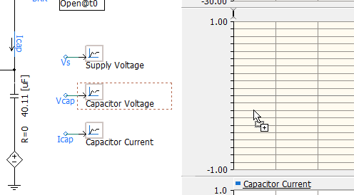
figure 30. Connect measurement to graph (Drag and drop while holding CTRL).
- You can modify both the
Graph Panecaption and theOverlay GraphY-axis title by double clicking on either the top title bar or on the overlay graph respectively and editing the appropriate parameter. Rename them something appropriate.
Sign-off
Once you are satisfied that you have collected all of the information required for your lab report get a lab instructor or TA to check your results and if everything is alright they will sign your sign-off sheet.
3.2.9 Postlab Graphs
G2. For the initial simulation conditions of the capacitor energization circuit include the plot of the Vs, Vcap and Icap waveforms in your lab report.
G3. For comparison, include the plot of the Vs, Vcap and Icap waveforms in your lab report for when the AC voltage source resistance is set to zero (ie. ideal).
G4. For another comparison, include the plot of the Vs, Vcap and Icap
waveforms in your lab report for when the source resistance is returned
to its original value of 0.1 Ω, but
Time of First Breaker operation is changed to 0.02084
seconds.
G5. For a last comparison, include the plot of the Vs, Vcap and Icap
waveforms in your lab report for when the source resistance is its
original 0.1 Ω and Time of First Breaker operation is
0.02084 seconds like the previous plot. However this time change the DC
voltage source that controls the pre-charge voltage of the capacitor to
28.17 kV.
3.2.10 Postlab Questions
Q3. For the plots obtained with the initial simulation conditions explain the behavior of waveforms before and after capacitor switching.
Q4. For the plots obtained with a AC source resistance of zero ohms, explain the difference in behavior of the waveforms compared to those with the initial simulation conditions.
Q5. For the plots obtained with the modified fault time of 0.02084 seconds, explain the difference in behavior of the waveforms compared to those with the initial simulation conditions.
Q6. Make the following measurements from the 2 separate scenarios when the breaker time is set to 0.02084 seconds. Note that these 2 different scenarios have the capacitor initially pre-charged to different values (0 kV and 28.17 kV).
The steady-state peak current of capacitor.
The highest transient peak current of capacitor.
The steady-state peak voltage of capacitor.
The highest transient peak voltage of capacitor.
Hint: in order to get the right steady state waveforms extend the simulation period to 0.5 sec.
Explain what the impact of pre-charged voltage of the capacitor has on the maximum transient current? Use yours measured results to back up your answer.
3.3 Back-to-back Capacitor Energization
In this task, the transient behavior of two capacitors energized sequentially is studied. In order to do this a new capacitor branch is paralleled with the capacitor branch of the system in the previous section. During the simulation after the first capacitor is charged, the second capacitor is then also switched onto the system and the resulting transient waveforms are studied. The Back-to-back capacitor energization circuit is shown in next figure.
Modify the existing circuit to obtain the Back-to-back capacitor energization circuit below.
Add a parallel branch to the previous circuit that includes a 19.2uH inductor, a timed breaker and a 22.29uF capacitor. Make sure to include meters to measure the new capacitors voltage and current.
Note that neither branch has a pre-charge DC power supply for the capacitor.
The timing for the breakers should be as follows.
- Both breakers should be configured as:
- Number of Breaker Operations = 1
- Initial State = Open
- BRK1 - Time of first breaker operation = 0.01667 s
- BRK2 - Time of first breaker operation = 0.037 s
- Both breakers should be configured as:
Create the required graphs so all of the meters can be plotted. Place all of the voltages in one
Graph Paneand all of the currents in another.
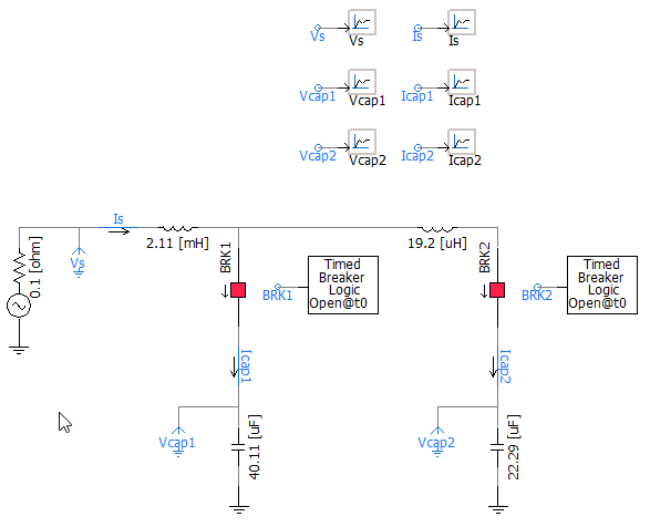
figure 31. Back-to-back capacitor energization.
Sign-off
Once you are satisfied that you have collected all of the information required for your lab report get a lab instructor or TA to check your results and if everything is alright they will sign your sign-off sheet.
3.3.1 Postlab Graphs
G6. For the back-to-back capacitor energization circuit include the plot of the Vs, Vcap1, and Vcap2 waveforms in your lab report.
G7. For the back-to-back capacitor energization circuit include the plot of the Is, Icap1, and Icap2 waveforms in your lab report.
3.3.2 Postlab Questions
Q7. Explain the behavior of the Vs, Vcap1, and Vcap2 waveforms before and after the switching of the second capacitor.
Q8. Explain the behavior of the Is, Icap1, and Icap2 waveforms before and after the switching of the second capacitor. Why are the peak current magnitudes of Icap1 and Icap2 so much larger than that of Is?
Q9. Go to the Project ribbon and change
Solution Time Step from 5 us to 100 us and run the
simulation again. What is the impact of solution time step on the
results? You may need to zoom in on the plots during the transient to
see the change of results clearly.
4 Postlab
Submit the following on eClass using the
Submit (Lab 5 - Results) link before the postlab due date.
Every student needs to hand-in their own results. Please merge all the
following into a single pdf document in the following order:
Use a scanned/picture copy of the
ECE433 - Lab 5 - Sign-offsheet as your cover sheet converted to pdf. Make sure your name, student ID, CCID and lab section are visible in the table at the top of the page and make sure that you have obtained the required signatures from your lab instructor or TA during your lab session.A pdf of the completed
ECE433 - Lab 5 - Postlabsheet including the required plots and answers to the postlab questions.
PDFsam Basic is a free and open source software that can be used for the pdf merge: https://pdfsam.org/download-pdfsam-basic/