Lab 4 - Transient Stability Simulation
ECE433 - Power Systems Stability and Transients
Electrical and Computer Engineering - University of Alberta

figure 1: Power Station
1 Introduction
The purpose of this experiment is to get you familiar with power system transient stability analysis using computer software tools. In this lab, you will learn the basic concepts of transient stability and associated assessment methods. Case studies will be performed for you to understand the nature of the power system transient stability behavior, including generator 'swing' characteristics and associated voltage and power oscillation dynamics. Through this lab, you will gain an improved understanding on the various factors that affect the transient stability of power systems.
1.1 Summary
Task 1 - PSAT Familiarization
Learn to load and view an example system file, complete a Power Flow simulation and then inspect and save the results in the software that is used for this lab.
Task 2 - Transient Stability Analysis
Complete a series of Time Domain simulations when adding a fault to one of the buses and changing the faults duration in order to determine the system’s critical fault clearing time.
Task 3 - Impact of Fault Location
Determine how a fault’s location impacts the critical fault clearing time of the system by running a series of Time Domain simulations with a fault on each one of the buses.
Task 4 - Impact of Line Tripping
Determine how removing a transmission line from the system impacts the critical fault clearing time for the system by comparing this case to the initial case.
Task 5 - Impact of Inertia
Determine how the inertia of a generator effects the critical fault clearing time of the system by comparing this case to the initial case.
1.2 Background
1.2.1 Power System Transient Stability
Transient stability is the ability of a power system to remain in synchronism when subjected to large transient disturbances. These disturbances may include faults on transmission elements, loss of load, loss of generation, or loss of system components such as transformers or transmission lines. Although many different forms of power system stability have emerged and become problematic in recent years, transient stability still remains a basic and important consideration in power system design and operation. While it is true that the operation of many power systems is limited by phenomena such as voltage stability or small-signal stability, most systems are prone to transient instability under certain conditions or contingencies and hence the understanding and analysis of transient stability remain fundamental issues. Also, transient instability can occur in a very short time frame (a few seconds), leaving no time for operator intervention to mitigate problems. It is therefore essential to deal with the problem in the design stage or severe operating restrictions may result.
Following a disturbance, synchronous machine frequencies undergo transient deviations from synchronous frequency and power angles change. The objective of transient stability study is to determine whether or not the machines will return to synchronous frequency with new steady-state power angles. In many cases, transient stability is determined using “swing curves” plotted for a generator subjected to a particular system disturbance. Trace “a” shown below shows that the generator power angle recovers and oscillates around a new equilibrium point. It is deemed to be transiently stable. However, in trace “b”, the power angle increases aperiodically and is considered transiently unstable. What factors determine whether a machine will be stable or unstable? How can the stability of large power systems be analyzed? If a case is unstable, what can be done to enhance stability? These are some of the questions to be solved in this lab.
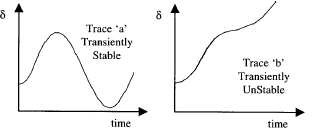
figure 2. Typical swing curves.
1.2.2 Methods of Transient stability Analysis
You have learned the theory of swing equation and equal area criterion in the lecture. It can be used to conduct analytical studies on small systems. For a practical system with large numbers of generators, transmission units and loads, the time-domain based simulation method is a more applicable approach.
For stability assessment, the power system is normally represented using a positive sequence model. The network is represented by a traditional positive sequence power flow model that defines the transmission topology, line reactances, connected loads and generation, and pre-disturbance voltage profile.
Generators can be represented with various levels of detail, selected based on such factors as length of simulation, severity of disturbance, and accuracy required. The most basic model for synchronous generators consists of a constant internal voltage behind a constant transient reactance, and the rotating inertia constant. This is the so-called classical representation that neglects the machine physical construction factors (damper windings, saturation, etc), the generation controls (excitation and governor systems) and the details of the prime mover. More detailed models have been utilized in commercial transient stability programs.
Transient stability studies are commonly performed after power flow studies. Based on the pre- disturbance system profiles, time-domain simulation can be conducted. The results are examined, usually through a graphical plotting, to determine if the system remains stable and to assess the details of the dynamic behavior of the system. Typical procedures for the transient stability analysis are as follows.
Collect data of network topology and power system components for power flow studies
one-line diagram of the network
transmission line and transformer data
shunt capacitors and reactors data
bus load data
generator real power output, scheduled voltage
Collect specified data for transient stability studies
Dynamic data: Includes model types and associated parameters for generators, motors, protections, and other dynamic devices and their controls.
Switching data: Includes the details of the disturbance to be applied. This includes the time at which the fault is applied, where the fault is applied, the type of fault and its fault impedance if required, the duration of the fault, the elements lost as a result of the fault, and the total length of the simulation.
Program control data: Specifies such items as the type of numerical integration to use and time-step.
System monitoring data: This specifies which quantities are to be monitored (output) during the simulation.
Solve power flow for the system
Perform transient stability studies
Perform time domain simulation.
Plot system swing curves to determine if the system remains stable.
Repeat the above process for different fault locations and different scenarios.
Document all study results
1.3 Required Software
The following software is installed on the computers that are provided in the laboratory. The following installation instructions are provided if you care to install the software on your own computers. It is your responsibility to get this working on your own hardware as little support will be provided by the laboratory staff as it can become too time consuming. Both Matlab/Simulink and the PSAT toolbox should be able to be installed on Windows, macOS and Linux.
1.3.1 Matlab/Simulink
MATLAB is a programming and numeric computing platform widely used by engineers and scientists to analyze data, develop algorithms, and create models.

figure 3. MATLAB and SIMULINK.
1.3.1.1 Installation Instructions
Create a Mathworks account using your University of Alberta email by visiting this link. https://www.mathworks.com/login
If you already have an existing account, simply login.
Note: It is important that you use your University of Alberta email when creating the account as this is how Matlab obtains its license.
Download the installer for your operating system for the recommended version of Matlab by clicking on the download icon in your Mathworks account.
- Recommended Version - Matlab 2019a
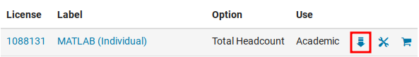
figure 4. My Software in your Mathworks account.
Install Matlab using the downloaded installer. When installing you only need to install Matlab and Simulink. There is no other toolbox required to run the lab other than the Power System Analysis Toolbox (PSAT) which is discussed below. I would only install the toolboxes you need as the toolboxes can be very large and can slow down your Matlab session. You can always add or remove toolboxes from within Matlab or by running the installer again.
Note: You will need to authenticate during installation using the Mathworks account you created in the first step to license Matlab properly.
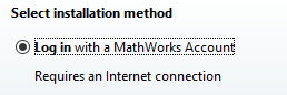
figure 5. Licensing install method.
1.3.2 PSAT
The Power System Analysis Toolbox (PSAT) is a Matlab toolbox for electric power system analysis and simulation.
figure 6. PSAT (Power System Analysis Toolbox)
1.3.2.1 Installation Instructions
Download the Power System Analysis Toolbox (PSAT) from the following link.
- Recommended Version - 2.1.11 - http://faraday1.ucd.ie/psat.html
Extract the downloaded
.zipfile to the Matlab toolbox directory atProgram files/MATLAB/R2019a/toobox/by default on Windows. There should be a similar directory for other operating systems.Add a PSAT toolbox installation path to the same directory that you extracted the toolbox too using the
Set Pathbutton on the toolbar in Matlab.
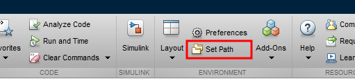
figure 7. Set PSAT toolbox path in MATLAB.
- Launch PSAT by typing
psatin the Matlab command window and after a few moments the PSAT control windows should be displayed as shown below.
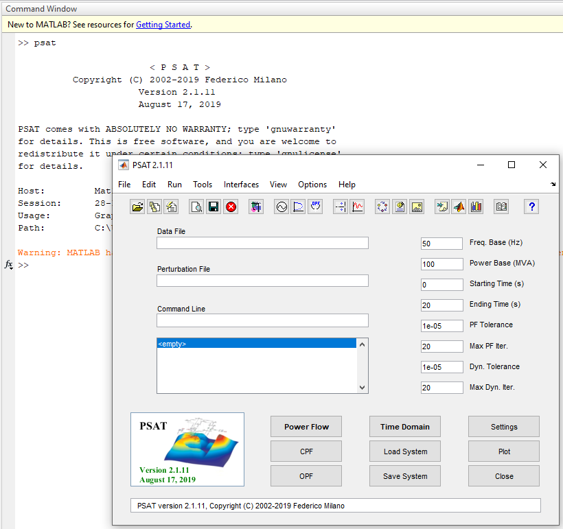
figure 8. PSAT main command windows.
2 Pre-lab
Please complete the following before attending your scheduled lab session.
2.1 Pre-lab Tasks
Make sure you know where and when to come to the lab by looking at the lab schedule that is available on eClass.
Familiarize yourself with the lab procedures and requirements by reading through the lab manual.
Complete the questions from the ECE433 - Lab 4 - Prelab Questions template. The same questions are shown below.
Have at least, the ECE433 - Lab 4 – Sign-off sheet printed off before coming to the lab.
Note that there is a ECE433 - Lab 4 - Postlab template for you to complete to hand in for submission. You will need to collect plots to include as images as well as complete the tables. The postlab questions are shown inline in the lab manual at the appropriate place as well as in the template.
2.2 Pre-lab Questions
What is transient stability? How does a transient instability manifest in a power system?
What are the main objectives of stability analysis?
Give the definition of swing curve. Explain what is the scenario of loss of synchronism?
What is the maximum real power output of a generator (simplified synchronous generator model) to an infinite bus?
Explain the equal area criterion.
List at least four factors that can influence transient stability. Explain how to manipulate these factors to improve the systems transient stability.
3 Lab Procedure
The system used for this experiment consists of 9 buses and 3 generating stations. It is so called WSCC 3-machine, 9-bus system and is widely used in power system transient stability studies. The system is shown in figure 9.
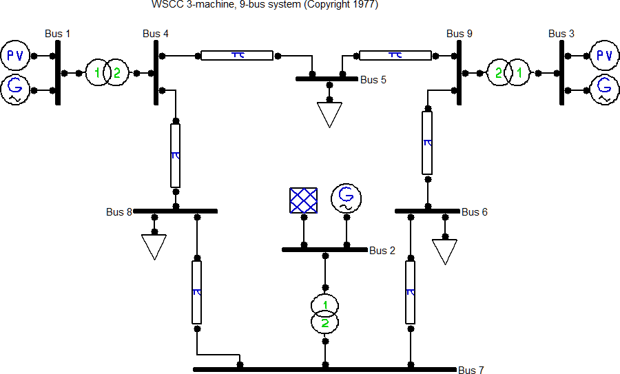
figure 9: The test system (The WSCC 3-machine, 9-bus system)
3.1 PSAT Familiarization
PSAT is a free Matlab toolbox for electric power system analysis and control. It includes power flow, continuation power flow, optimal power flow, small signal stability analysis and time domain simulation. All operations can be assessed by means of graphical user interfaces (GUIs) and a Simulink-based library provides a user friendly tool for network design.
3.1.1 Load the Basecase
- Download the .zip file from below which contains the Base Case that
will be used for this lab and extract it somewhere you can find in your
user space. It is usually easiest if you put the file in your default
Matlab workspace. The extracted .zip file contains a single .mdl file
titled
Lab_4_Basecase.mdl.
Base Case Download
- In the PSAT command window click on the
Open Data Filebutton as shown below or navigate the menus toFile/Open/Data File.
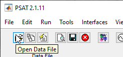
figure 10. Open Data file button.
From the opened Load Data File screen, navigate the directory structure to where you have the .mdl file extracted. Make sure that the Filters is to
PSAT Simulink (.mdl)and select the correct Basecase file underFiles in current path:and then click on theLoadbutton.Note: The mdl file contains the single-line 9-bus system diagram in a Simulink file format which was constructed with the PSAT simulink library. When we
Load Data file, PSAT extracts the data from the Simulink and creates another file which ends with a.m, which it then uses in its simulation calculations. You can review some of this conversion process in the Matlab Command Window.
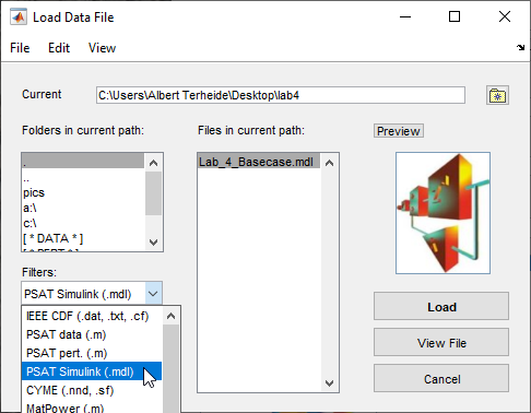
figure 11. Load a simulink .mdl file into the PSAT toolbox for analysis.
To view and/or edit the single-line diagram of the system in Simulink, you can go to
File/Open/Simulink Modeland open the same downloaded .mdl file.Note: If you make changes to the Simulink model you need to first save the new model in the .mdl format and then make sure that you
Load Data filein PSAT before carrying out any simulation.Note: The Simulink library blocks may have an Unrecognized functions or variables error and are highlighted in red. As we are not using the Simulink solver this does not matter. If the red highlight bothers you, you can try simulating the model in Simulink, nothing will really simulate but it will create the missing variables and the errors will go away.
Note: You can double click on the blocks in the model to edit their
Block Parameters.
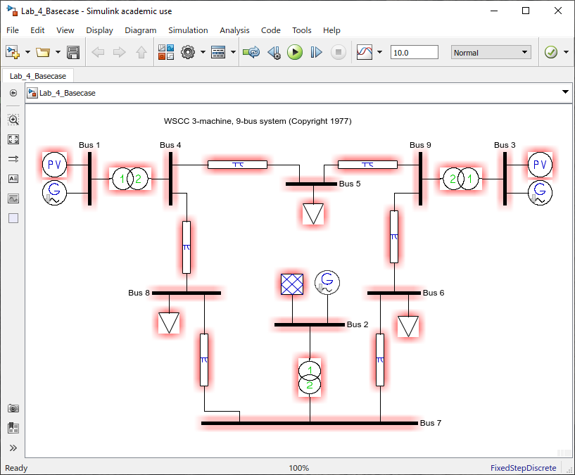
figure 12. An open .mdl file in Simulink where the system can be edited.
- Change the system frequency to 60 Hz in the main PSAT window as this is the typical system frequency in North America, it defaults to 50Hz as the PSAT software is written somewhere in Europe where that is the typical system frequency.
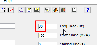
figure 13. Change the system base frequency to 60Hz.
3.1.2 Simulate the Basecase
- To complete a Power Flow Analysis of the system press the “Power Flow” button in the PSAT main window, the status of the simulation gets logged in the Matlab Command Window.
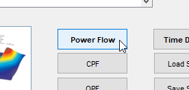
figure 14. Complete a Power Flow Analysis of the System.
- Press the button shown below to view the Static Report of the Power Flow Analysis results.
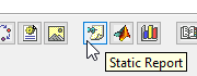
figure 15. Open the Static Report of the Power Flow Analysis.
An example of the Static Report results are shown below.
Note: In the upper parameter boxes the highlighted entries indicate the values of the selected bus.
Note: You can change the units displayed in the boxes by clicking on the unit displayed at the top of each box.
Note: For Active and Reactive Power you can also select where to display the following
- G - The generated power on the bus.
- L - The comsumed power on the bus.
- I - Shows both: generated as a positive number and consumed as a negative number.
Note: You can click on the icon to open up a bargraph plot to compare the results of each bus.
Note: You can generate/save a Static Report by pressing on the Report button. The report output format and other options can be configured by selecting what you want under the
Preferences Menu.
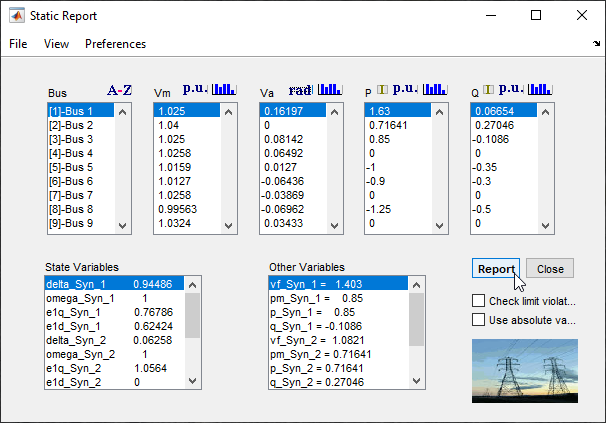
figure 16. An example Static Report.
3.1.3 Basecase results
- Compare your Power Flow Analysis results in the Static Report with the reference results shown below.
| Bus # | Voltage (pu) | phase (°) | P_gen (pu) | Q_gen (pu) | P_Load (pu) | Q_Load (pu) |
|---|---|---|---|---|---|---|
| 1 | 1.02500 | 9.28000 | 1.63 | 0.06654 | — | — |
| 2 | 1.04000 | 0.00000 | 0.71641 | 0.27046 | — | — |
| 3 | 1.02500 | 4.66480 | 0.85 | -0.1086 | — | — |
| 4 | 1.02580 | 3.71970 | — | — | — | — |
| 5 | 1.01590 | 0.72754 | — | — | 1 | 0.35 |
| 6 | 1.01270 | -3.68740 | — | — | 0.9 | 0.3 |
| 7 | 1.02580 | -2.21680 | — | — | — | — |
| 8 | 0.99563 | -3.98880 | — | — | 1.25 | 0.5 |
| 9 | 1.03240 | 1.96670 | — | — | — | — |
- Change the Report output format to Excel by going to
Preferences/Select Test Viewerand selectingExceland clicking on OK. Generate the Report and Save it with an appropriate name. Have a look at the report to see what is included.
3.2 Transient Stability Analysis
Transient stability examines the impact of disturbances on power systems considering the operating conditions. The analysis of the dynamic behavior of power systems for the transient stability gives information about the ability of a power system to sustain synchronism during and after a disturbance.
In this task, a fault will be placed on one of the buses to demonstrate how the system behaves. A system can recover if a fault is cleared quickly enough before the whole system collapses.
Add a fault to bus 4 by doing the following.
- With the Simulink model of the system open also open the PSAT simulink library by clicking on the appropriate button in the PSAT main window.
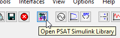
figure 17. PSAT Simulink library button.
- In the base case Simulink model, double click on bus 4 (the thick
black line) to open the
Block Parameterwindow for Bus 4. Change theNumber of outputs:from 2 to 3. You will then see another output appear on the bus 4 in the Simulink model.
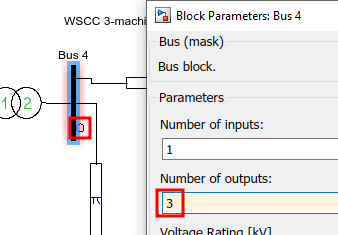
figure 18. Adding a new output on bus 4.
- From the PSAT Simulink library, either drag and drop or copy and
paste a
Fault(from the Faults and Breakers library) to your base case some where near bus 4.
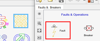
figure 19: Faults and Breakers catalogue of the PSAT Simulink library.
- Wire the newly added Fault to the new output your created on bus 4.
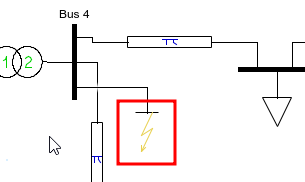
figure 20: Connect the new Fault to bus 4.
Double click the fault and setup the following parameters:
- Power, voltage and frequency: [100 230 60]
- Fault time: 1.0
- Fault clearing time: 1.15
Note: The duration of the fault will be the
Fault clearing timeminus theFault timeas both of the times above are the times in the simulation that the events occur.Save this new case with a new appropriate name making sure to save it as an .mdl file so it can be loaded into PSAT.
Load the new .mdl Data File you just created by clicking on the
Open Data Filebutton in the PSAT main window. Make sure to adjust the file typeFilterso.mdlfiles can be seen.Go to Settings in the PSAT main window and check the selection of
Convert PQ bus to Zto increase the simulation’s stability.
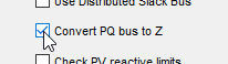
figure 21: Convert PQ bus to Z.
- Run a Time Domain simulation in PSAT by clicking on the button shown below. The Time Domain solution requires an initial Power Flow solution before it is run and it will do it automatically if a current solution is not available.
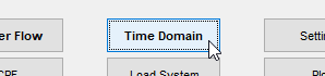
figure 22: Run a Time Domain simulation.
Using the PSAT
Plot tool, plot the following and save the resulting graphs using a screen capture tool likeSnip & Sketchto save the plot as an image file to include in your Postlab.Note: The first 3 plots below have a fault clearing time of 0.15s.
Note: You can change the length of the simulation from the PSAT main window as shown below.
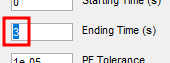
figure 24. Simulation End Time.
Note: You can examine the resulting waveforms in more detail by using the plots zoom controls.
- Power Angle at Generator Buses: Select the power
angle (δ) of the 3 synchronous generators (ie. delta_Syn_1) to plot them
against time. Use delta_Syn_1 as reference angle by selecting it in the
appropriate box. Click on the
Plotbutton to generate the graph in the available space. Use the default simulation end time of 20 seconds.
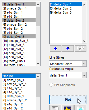
figure 23. Select the parameters that you would like to plot. The power angles of the 3 generators shown.
Voltage at Generator Buses: Select the bus voltages that the 3 synchronous generators are attached to (ie. V_Bus 1) to plot them against time. Click on the
Plotbutton to generate the graph in the available space. Change the simulation end time to 3 seconds (or use the Zoom tool) so what is occuring to the voltages during the fault can be seen.Power at Generator Buses: Select the 3 synchronous generator power quantities (ie. p_Syn_1) to plot them against time. Click on the
Plotbutton to generate the graph in the available space. Change the simulation end time back to 20 seconds.Unstable - Power Angle at Generator Buses: The longest fault time duration that the system can recover from and remain stable is named as critical fault clearing time. Run the simulation while increasing the fault duration by 0.01 second increments to find the critical fault clearing time for bus 4. Record the critical fault clearing time in the appropriate places in the results table and plot the power angle (δ) of the 3 generators when the system goes unstable.
- Power Angle at Generator Buses: Select the power
angle (δ) of the 3 synchronous generators (ie. delta_Syn_1) to plot them
against time. Use delta_Syn_1 as reference angle by selecting it in the
appropriate box. Click on the
Sign-off
Once you are satisfied that you have collected all of the required plots in an image format for your lab report, show them to a lab instructor or TA for them to sign on your sign-off sheet in the appropriate place.
3.2.1 Postlab Questions
Q1. Is the system stable? Explain why.
Q2. Explain what is occurring in the generator plots for both the voltage and the power, that you obtained, when a fault is applied to bus 4 between 1.0 to 1.15 seconds of the simulation.
3.3 Impact of Fault Location
The amount of time a fault is sustained before the system collapses can vary depending on where in the system the fault occurs. Therefore the system’s critical fault clearing time should be different if a fault occurs in a different location (ie. on a different bus).
Using a similar procedure as the previous section to complete the table below, determine the systems critical fault clearing time when a single fault occurs at each of the 9 buses. Record your results in the table provided on your results sheet.
Note: You already completed bus 4 in the previous section.
| Bus # | Bus Voltage (kV) | Critical fault clearing time (s) |
|---|---|---|
| 1 | 18.0 | |
| 2 | 16.5 | |
| 3 | 13.8 | |
| 4 | 230.0 | |
| 5 | 230.0 | |
| 6 | 230.0 | |
| 7 | 230.0 | |
| 8 | 230.0 | |
| 9 | 230.0 |
Note
It is important that the fault voltage rating matches the voltage rating of the bus.
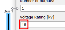
figure 25. The rated bus voltage.
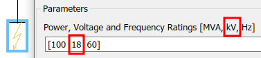
figure 26. The rated fault voltage.
Sign-off
Once you are satisfied that you have collected all of the critical fault clearing times required for your lab report get a lab instructor or TA to check your results, and if everything is alright they will sign your sign-off sheet.
3.3.1 Postlab Questions
Q3. Which fault location is most susceptible to cause a system transient that will lead to an unstable system? What are the potential reasons for that?
Q4. Explain why doing a fault location scan, like was completed in the lab, could be useful.
3.4 Impact of Line Tripping
If a circuit breaker protecting a transmission line trips either before or during a fault event the critical fault clearing time will be effected.
For this case, we will start with the same case that we used in the
Transient Stability Analysis where we had a fault on bus 4.
However for this new case we will add a breaker in the line from bus 7
to bus 8 that will open before the fault occurs and then close again
after the fault transient has subsided. The goal of this task is to see
how a change in the system effects the critical fault clearing time.
Add a Breaker to the line from bus 7 to bus 8 by doing the following.
Open the
.mdlfile that you saved in theTransient Stability Analysessection where you just added a fault on bus 4 into Simulink. As this is the case we want to compare to.Open the PSAT Simulink library and copy a
Breakerfrom theFaults & Breakerscatalogue someone near either bus 7 or bus 8 in your base case.
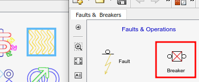
figure 27. A Breaker in the Faults and Breaker catalogue of the PSAT Simulink library.
- Delete the wire connecting the bus to the line element and place the new Breaker in series with the line by wiring the breaker to both the line element and the appropriate bus.
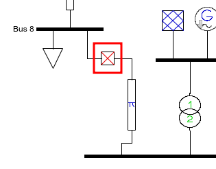
figure 28. A breaker inserted in series with the line that connects bus 7 to bus 8.
- Double click on the
Breakerelement and theBlock Parametersfor theBreakerwill open. Set the parameters as shown below.
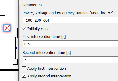
figure 29. The breakers parameter settings.
- Save the new case with a new appropriate name as a
.mdlfile.
Load the newly saved file into PSAT using the PSAT command window.
Like you did in the previous sections, determine the system’s new critical fault clearing time when the newly added Breaker is open. Record your results in the table provided on your results sheet.
Sign-off
Once you are satisfied that you have the correct critical fault clearing time for your lab report get a lab instructor or TA to check your results, and if everything is alright they will sign your sign-off sheet.
3.4.1 Postlab Questions
Q5. How does a line being removed from the system effect the systems transient stability? Explain.
3.5 Impact of Inertia
The inertia of a generator will effect how fast the power angle changes when a transient occurs which means that it will either take longer or shorter for that generator to reach the point of instability depending if the inertia is increased or decreased.
For this case, we will again start with the same case that we used in
the Transient Stability Analysis where we had a fault on
bus 4. However for this new case we will increase the inertia of all
three of the generators of the system to demonstrate its effect on the
critical fault clearing time.
For this test we are going to double the inertia of all three of the generators in the system. Follow the steps below to change the inertia of a generator.
Start again by reopening the
.mdlfile that you saved in theTransient Stability Analysessection where you just added a fault on bus 4 into Simulink. As this is the case that we want to compare to.Double click the generator to open the
Block Parameterwindow. Double theInertiavalue that is shown below.Note: You can use math in the parameters so you can simply add a 2* infront of the inertia parameter to double it.
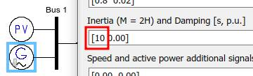
figure 30. Setting the Inertia of a generator.
Modify all 3 generators so that their inertia is doubled.
Save the new case with a new appropriate name as a
.mdlfile.
Load the newly saved file into PSAT using the PSAT command window.
Like you did in the previous sections, determine the systems new critical fault clearing time when the systems generators inertia are all doubled. Record your results in the table provided on your results sheet.
Sign-off
Once you are satisfied that you have the correct critical fault clearing time for your lab report get a lab instructor or TA to check your results, and if everything is alright they will sign your sign-off sheet.
3.5.1 Postlab Questions
Q6. How does the inertia of all of the generators in the system effect the systems transient stability? Explain.
4 Postlab
Submit the following on eClass using the
Submit (Lab 4 - Results) link before the postlab due date.
Every student needs to hand-in their own results. Please merge all the
following into a single pdf document in the following order:
Use a scanned/picture copy of the
ECE433 - Lab 4 - Sign-offsheet as your cover sheet converted to pdf. Make sure your name, student ID, CCID and lab section are visible in the table at the top of the page and make sure that you have obtained the required signatures from your lab instructor or TA during your lab session.A pdf of the completed
ECE433 - Lab 4 - Postlabsheet including the required plots, completed tables and answers to the postlab questions.
PDFsam Basic is a free and open source software that can be used for the pdf merge: https://pdfsam.org/download-pdfsam-basic/