Lab 3 - Voltage Stability Accessment
ECE433 - Power Systems Stability and Transients
Electrical and Computer Engineering - University of Alberta

figure 1: A Power Station.
1 Introduction
Voltage stability is concerned with the ability of a power system to maintain acceptable voltages at all buses in the system under normal conditions and after being subjected to a disturbance. It is an important consideration in the design and operation of power systems. In this lab, you will learn the basic concepts of voltage stability and associated assessment methods. Case studies will be performed to understand the P-V and Q-V characteristics of a power system under different circumstances. Through this lab, you will gain an understanding on the various limiting factors that affect the capability of a power transmission system to transport power to loads.
1.1 Summary
Task 1 - Create P-V Curves - Base Case
Starting with the original system the P-V curves for each load bus will be determined. To do so both the real and reactive power load demand will be proportionally scaled up in increments while the total system load and the bus voltages are recorded. At some point the load will become too great for the system and the system will go into Blackout at its limit.
Task 2 - New Transmission Line
The base case will be modified by placing an identical parallel transmission line between two of the buses in order to decrease the impedance between the two buses. The P-V curves of this case and the base case will be compared to demonstrate the effect of the new parallel transmission lines effect on the systems performance.
Task 3 - Limiting Reactive Power Capacity
The base case will again be modified to include a reactive power output limit on the generator at bus 2 which the generator will hit during the experiment. The P-V curves of this case and the base case will be compared to demonstrate the effect this limit on the systems performance.
Task 4 - Impact of Shunt Capacitor
This case will use the previous case as its starting point and also disconnect the shunt compensation capacitor on bus 4 which will increase the reactive power needed to be supplied by the generators. The P-V curves of this case and the other cases will be compared to demonstrate the effect removing the shunt compensation capacitor has on the systems performance.
Task 5 - Create Q-V Curves
Starting from the Base Case we are going to determine the Q-V curve at bus 9 using 2 different approaches so they can be compared. The first approach is to attach a temporary generator as a synchronous condenser to the bus under test to control its voltage and then measure the reactive power consumed by the generator. In the second approach the reactive power is increased using a reactive load on the bus under test and measuring the resulting bus voltage. ***
1.2 Background
1.2.1 The Voltage Stability Problem
Voltage stability is also called the load stability. It is a characteristic of a power system that is required to transmit sufficient power to meet load demand. The voltage stability is the ability of the system to maintain acceptable voltage at all buses in the system under normal and abnormal operating conditions. A power transmission network has an inherent limit as to how much power it can deliver to loads. When this limit is exceeded, the voltages experienced by loads become too low to be practically useful. In many cases, the voltages will go straight from normal to zero in a matter of a few seconds or minutes. This process is called voltage collapse. Massive voltage collapses across several interconnected power systems are not unusual. For example, at the summer of 1996, two voltage collapses occurred in the west coast Canada- US-Mexico interconnected system, causing blackouts for millions of customers.
The capability of a transmission network can be loosely visualized as the size of a pipe or the number of parallel pipes. The power transfer capability of this system would be affected if one or more pipes (transmission lines) are lost. Loss of transmission lines or other supporting components such as shunt capacitors will cause the reduction of system capability. When system capability is reduced, loads have to be shed. Otherwise the demand and supply cannot match and voltage collapse will occur.
The simplest form of voltage stability assessment involves the determination and characterization of a network’s power transfer capability. This capability must be greater than the anticipated load. The network
capability will change if some of its components are not available due to failure or maintenance. The capability assessment therefore needs to be conducted for a number of contingency scenarios for planning and managing the system. P-V and Q-V curves are two most commonly used techniques to assess the capability of a network. These curves show the voltages of selected buses as functions of increased system load. The “nose points” of these curves are the system limit.
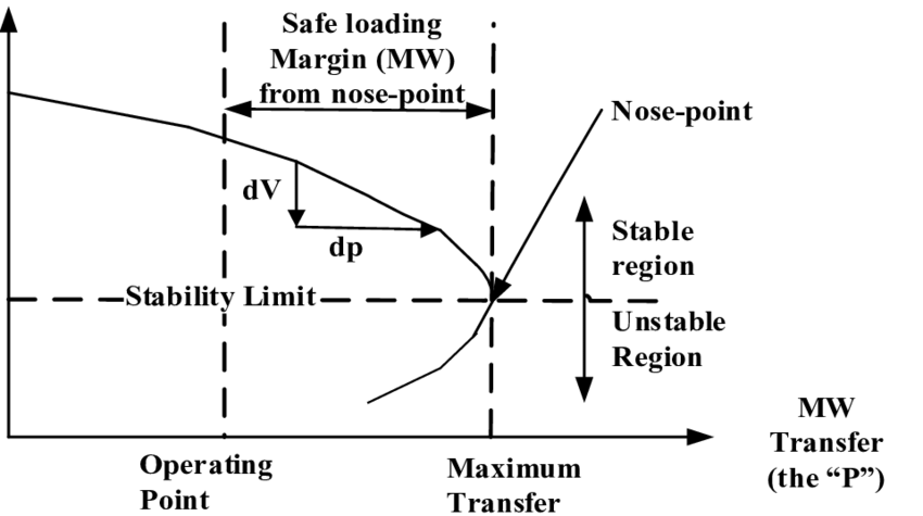
figure 2. A typical P-V curve.
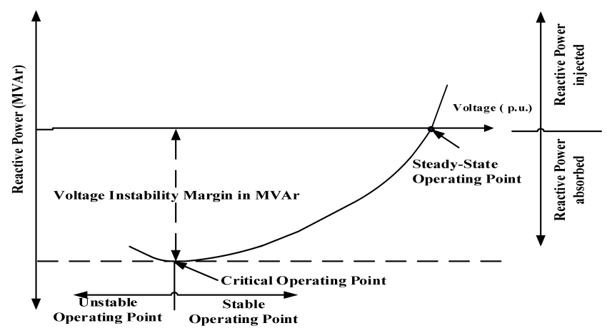
figure 3. A typical Q-V curve.
1.2.2 Voltage Stability Analysis
In this lab, voltage stability analysis is just limited to the assessment of system capability using P-V and Q-V methods. The capability will be determined for various operating scenarios. The results will help you to understand what are the impact factors that affect network transfer capability and hence the voltage stability of a system.
1.2.3 P-V Curve
The P-V curve method is a process to determine the P-V curves of a network. While there are many advanced and automated methods to determine the curves, the following procedure is sufficient to determine simple P-V curves of a network:
P-V Curves Procedure
Develop a load flow base case. The case, reflecting existing system loading and operating conditions, must be solved successfully by your load flow program (The PowerWorld Simulator).
All loads (both real and reactive power parts) in the system are scaled to a new level. The generator output may also need to be scaled. In this lab, generation scaling is not performed to simplify the process. Thus, the power mismatch is supplied by the slack generators. Record the new total load level, as P1 (the real power part).
The case is solved by using the load flow function again. If the case solves, record the voltages of key buses (called monitored buses) as VA1, VB1 … etc. If the case cannot be solved or diverges, go to step 6.
Save the solved case. Scale up the loads again on the basis of this solved case and solve it. If it solves, record the results as P2, and VA2, VB2 … etc.
Steps 2 to 4 are repeated until the case cannot be solved, i.e. the solution of load flow diverges.
If the load flow diverges, it typically means that the limit (nose-point) has been reached. The P-V curve process is now completed. The results, recorded P and V data points, can be plotted as P-V curves.
It is important to note the following points:
The amount of load increase should be gradually decreasing as one approaches the nose point. Namely, the incremental P becomes smaller and smaller. The purpose is to help one to zero in the nose point more accurately.
When solution diverges, don’t record the results. The output results are not correct.
The P-V curve plots V against P, although the system Q has also been changed in proportion to P. The exact name for P-V curve should therefore be the SV curve. However, the terminology of P-V curve has been accepted in industry. P-V curve does not mean to increase P only.
1.2.4 Q-V Curve
The Q-V curve method is a process to determine the Q-V curves of a network. A Q-V curve represents the system voltage behavior when increased reactive power is withdrawn from a bus called test bus. This is done by connecting a synchronous condenser (a generator with zero active power) to the test bus. The voltage setting of the condenser is decreased gradually, resulting increased withdrawal of reactive power from the network. There is a limit for the amount of reactive power that can be withdrawn. This limit is the nose point. The process of obtaining a Q-V curve is as follows:
Q-V Curves Procedure
Develop a solved load flow base case.
Select the test bus. Test bus is typically an important bus in the network. The need to select a test bus is one of the main drawbacks of the Q-V method. Record the test bus voltage.
Add a synchronous condenser to the test bus. A condenser has a zero P output. The voltage setting of the condenser is equal to the test bus voltage recorded in step 2.
Run the load flow. The case should be easily solved. Examine the output of the condenser. It should be zero for both P and Q. Save the case.
Decrease the voltage setting of the condenser by a small amount, say, 0.03pu. Run the load flow case. If the case is solved, record the Q output from the condenser. The output should be negative, indicating Q withdrawal from the system. Save the case.
If the case can not be solved, stop. Otherwise, repeat Step 5.
The above process will result in a series of data points (V1, Q1), ... (Vn, Qn). Plot of the Q data versus V data is the Q-V curve. In the Q-V curve method, one only records and charts the voltage and reactive power output of the test bus.
2 Pre-lab
Please complete the following before attending your scheduled lab session.
2.1 Pre-lab Tasks
Make sure you know where and when to come to the lab by looking at the lab schedule that is available on eClass.
Familiarize yourself with the lab procedures and requirements by reading through the lab manual.
Complete the questions from the ECE433 - Lab 3 - Prelab Questions template. The same questions are shown below.
Have at least, the ECE433 - Lab 3 – Sign-off sheet printed off before coming to the lab.
The ECE433 - Lab 3 - Spreadsheet will be used to record your results for analysis and submission.
Note that there is a ECE433 - Lab 3 - Postlab Question template for you to complete as part of your postlab. The same question are shown inline in the lab manual at the appropriate place.
2.2 Pre-lab Questions
What is voltage stability? How does voltage instability manifest in a power system?
What are the main objectives of stability analysis?
Give the definitions of P-V curve and Q-V curve. Why there is a "nose point" in these curves?
List at least four compensating devices or methods that can be used to maintain or to increase system voltage stability. Explain the advantages and disadvantages of each.
Plot qualitative P-V curves (in one chart) for the following cases:
- base case
- if a parallel line is added to an existing line
- if a shunt capacitor is added to the system
- if a series compensation is added to a line.
If a shunt capacitor is switched off in an industry plant, what could happen to the bus voltages? Use P-V curve to explain your answer.
State the advantages and disadvantages of the Q-V curve method.
If the reactive power output from a generator reaches its limit, will the generator help voltage stability? Explain why.
3 Lab Procedure
The system for this lab is the same as the one that was used in the previous lab titled Lab 2: Power Flow Calculations. You will experiment with this system focusing on a few voltage stability analysis tasks. You can download the base case below as a starting point for this lab.
Base Case Download
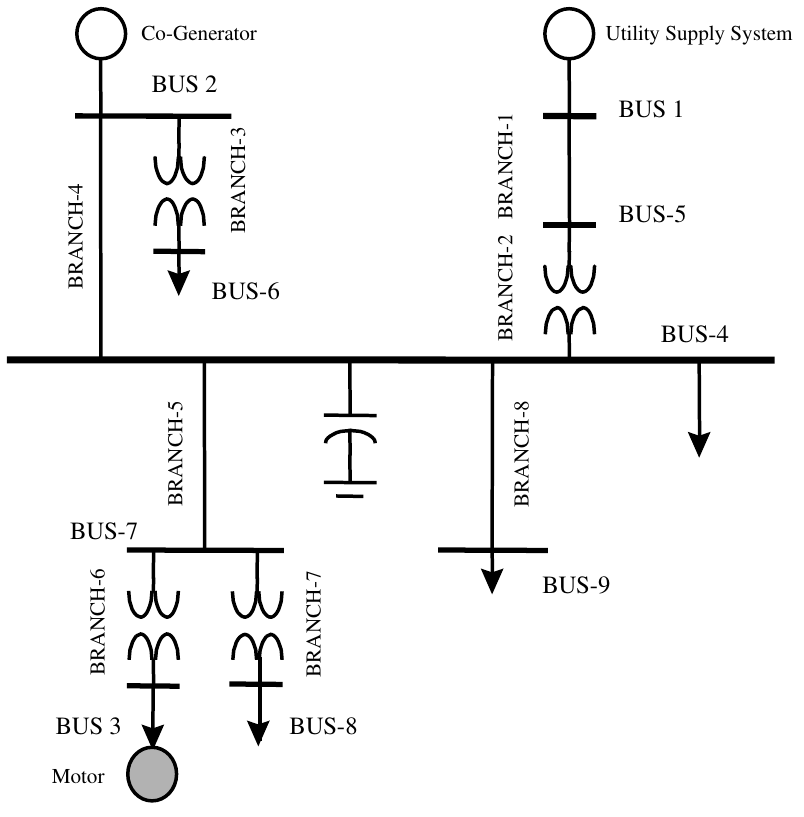
figure 4. A balanced industrial system.
3.1 How to Scale a Case
The simulator has a tool to that allows you to easily scale multiple
elements in the system by selecting the buses that the element is
attached to. An element can be a load, a bus shunt, or a generator that
is connected to one of the buses. The tools dialog box is shown below.
To open the scaling tool, under the Tools ribbon select
Scale Case in the Other Tools ribbon
group.
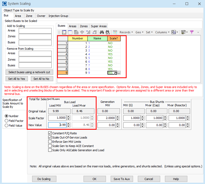
figure 5. The Scale Case tool.
The tool allows you to scale multiple objects proportionally by selecting the connected buses and entering the desired scaling value. You can either select buses directly or by there assigned Area, Zone, Super Area, Owner or Injection Group. We will be selecting the buses to scale directly.
For the lab, We want to increase the combined system load by scaling
all of the selected buses proportionally to achieve the desired loading
result. As we increase the loading on the system the voltages on the
buses will decrease until they are unable to supply the power to the
load and the system goes into a BLACKOUT. We do not scale
up the generation in order to simplify the procedure. Follow this
procedure when required to scale the buses.
Start by making sure the
BusandBusestabs are selected. In theBusesarea, the buses of the system are all listed and will initially all be set toNOmeaing that they will not be scaled For this lab we want to scale all of the load buses, therefore we can change buses 4, 6, 8 and 9 toYESto indicate they are the ones we want to scale.The total load of the selected buses will now be shown in the
Original Valuebox under theBus Loadheading. The original load should initially be 9.99 MW and 8.46 Mvar.Make sure the checkboxes at the bottom of the page are setup as follows:
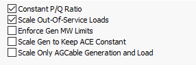
figure 6. Scale Case checkboxes.
To scale the selected buses the software allows you to do this in 2 ways: Either place a multiplier in the
Scale Factorbox to obtain new load values for each selected bus based on that multiplier, or place a new total load value for all selected buses in theNew Valuebox and the software will calculate how much it should add to each bus. Note that when I enter a value into one of the boxes the other value is calculated automatically once I hitEnter. Also note that the Q values also get scaled accordingly as we have theConstant P/Q Ratiocheckbox selected. The scaling of the system will not happen until theDo Scalingbutton is pressed at the bottom of the page.To make our simulations go a little more smoothly we can change a couple of the
Simulator Optionsunder theToolsribbon.Under
Power Flow Solution/Advanced Options/Power Flow (Inner) Loop OptionsSet theMinimum Per Unit Voltage for/Constant Power Loadsto0.00. This will ensure that simulation will run until the system goes toBlackoutinstead of stopping when one of the buses reaches this value.Just above the last setting also make sure to un-check the item
Initialize from Flat Start Values. This allows the system to automatically re-start the simulation from known values once the system goes intoBlackout.
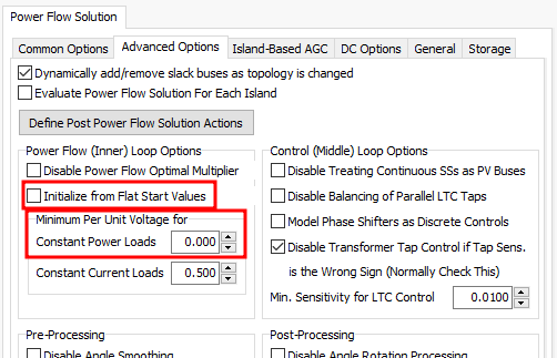
figure 7. Simulation Options.
3.2 Create P-V Curves
In this case, in order to determine the P-V curves for each load bus,
both the real and reactive power load demand will be scaled up in
increments until the system goes into Blackout. This is
done one power step at a time using the Scale Case tool
which is described in the How to Scale a Case section at
the beginning of the lab procedure.
Solve the
Base Caseto determine the initial per-unit voltages of all of the load buses (Bus 4, Bus 6, Bus 8 and Bus 9) at the initial system load demand. Record these values in the appropriate table on theECE433 - Lab 3 - Spreadsheet.Use the
Scale Casetool to increase the total load demand (both active power and reactive power) by proportionally increasing the load at each one of the buses so the total active power matches the required values in the table below. Determine the per-unit voltages of all of the load buses (Bus 4, Bus 6, Bus 8 and Bus 9) at each power setting and record these values in the corresponding table on theECE433 - Lab 3 - Spreadsheet. Note that every time youDo Scalingyou need to find the new solution by either clicking on theSolve Power Flow - Newtonbutton or by continuously running the solution by clicking on thePlaybutton in theToolsribbon.
| P (MW) | Bus 4 | Bus 6 | Bus 8 | Bus 9 |
|---|---|---|---|---|
| 9.99 | ||||
| 20 | ||||
| 30 | ||||
| 40 | ||||
| 50 | ||||
| 60 | ||||
| 70 | ||||
| ? | ||||
| 80 | BLACKOUT | BLACKOUT | BLACKOUT | BLACKOUT |
- Once the case diverges the following window will appear which
indicated that the system is now in Blackout and that the system can no
longer supply the load. Note that the system should solve up to 70 MW
but Blackout at 80 MW. Find the largest value between 70 and 80 MW, to 1
decimal place, where the system still solves without a Blackout and
record both the power and per-unit bus voltages in the corresponding
table on the
ECE433 - Lab 3 - Spreadsheet.
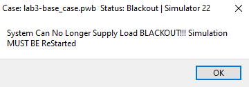
figure 8. BLACKOUT!!! popup.
Sign-off
Get a lab instructor or TA to check your results so far to see if you are on the right track, if everything is alright they will sign your sign-off sheet.
3.2.1 Postlab Questions
Q1. Why software should initialize from flat start for this study?
Q2. The P-V curves can be plotted for different buses. Do all curves have the same nose point? Why?
Q3. If only active power is scaled up in the process, one can get another set of 'P-V' curves. Draw qualitatively (no simulation is needed, draw based on your theoretical expectation) the following two curves in one chart and explain the difference: the first curve is the standard P-V curve, and the second curve is the P-V curve with only P scaled up. Please remember that you have to find more scaling factors for active power by trial and error until the case diverges.
3.3 New Transmission Line
In this section, starting with the base case, a second identical transmission line is added in parallel to the transmission line of branch 4. This changes the total impedance of branch 4 to be half of the original. The P-V curves will also be determined for this new case to compare to the previous case.
- Using the original base case, create a new transmission line in
parallel with the existing transmission line of branch 4. Make sure that
the
Per Unit Impedance Parametersare set to be equal to the existing transmission line. After making the required modification to the base case and solving it, save the new case with an appropriate name.
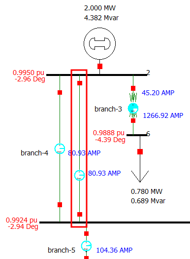
figure 9. An added second parallel transmission line.
- Use a similar procedure that you used in the previous section to
obtain the per-unit bus voltages when the load buses are proportionally
scaled up to the active powers listed in the table below. Record these
values in the corresponding table on the
ECE433 - Lab 3 - Spreadsheet.
| P (MW) | Bus 4 | Bus 6 | Bus 8 | Bus 9 |
|---|---|---|---|---|
| 9.99 | ||||
| 20 | ||||
| 30 | ||||
| 40 | ||||
| 50 | ||||
| 60 | ||||
| 70 | ||||
| ? | ||||
| 80 | BLACKOUT | BLACKOUT | BLACKOUT | BLACKOUT |
3.3.1 Postlab Questions
Q4. What is impact of adding a parallel line to the system P-V curve?
Q5. Why does adding a parallel line mean the line impedance is halved? If a line has a shunt admittance (the shunt branch of the common PI circuit for a line), what is the impact of adding a line on the admittance?
Q6. Are there other methods to reduce the line series impedance? (Name at least one)
3.4 Limiting Reactive Power Capacity
In this section, again starting with the base case, a reactive power output limit is going to be placed on the generator at bus 2 to demonstrate what the effect is. This would be a typical limitation of a actual generator. The P-V curves will also be determined for this new case to compare to the previous cases.
Note
Before starting this task open the Simulation Options to
verify that the reactive power limit of the generator will be taken into
consideration by the Simulator. To do this make sure that the
Disable Checking Gen VAR Limits is unchecked as shown
below.
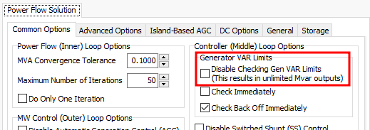
figure 10. Simulator Options.
- Using the original base case, change the
Max Mvarsetting of the generator at bus 2 to 46.8 MVar as shown below. After making the required modification to the base case and solving it, save the new case with an appropriate name.
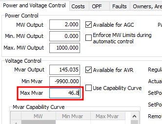
figure 11. Setting the generators maximum reactive power.
- Use a similar procedure that you used in the previous sections again
to obtain the per-unit bus voltages when the load buses are
proportionally scaled up to the active powers listed in the table below.
Record these values in the corresponding table on the
ECE433 - Lab 3 - Spreadsheet.
| P (MW) | Bus 4 | Bus 6 | Bus 8 | Bus 9 |
|---|---|---|---|---|
| 9.99 | ||||
| 20 | ||||
| 30 | ||||
| 40 | ||||
| 50 | ||||
| ? | ||||
| 60 | BLACKOUT | BLACKOUT | BLACKOUT | BLACKOUT |
3.4.1 Postlab Questions
Q7. Are there any differences in system voltages between the new base case of this study and the base case used in Task 1? Why?
Q8. What is the impact of generator Q limit on system capability? Explain.
Q9. Why does a generator have a limit for reactive power output (think your EE332 course)?
3.5 Impact of Shunt Capacitor
In this section, this time starting with the case from the previous Limiting Reactive Power Capacity section, the shunt capacitor at bus 4 is going to be turned off to demonstrate what the effect is. The P-V curves will also be determined for this new case to compare to the previous cases.
Note
Double check that the reactive power Limit of the generator will be taken into consideration.
- Using the case from the previous Limiting Reactive Power Capacity section, switch off of the capacitor at bus 4 by a clicking on the attached switch; The switch will go from being red to turning white with a green outline indicating its open status as shown below. After making the required modification to the base case and solving it, save the new case with an appropriate name.
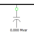
figure 12. Disconnecting the shunt compensation capacitor.
- Use a similar procedure that you used in the previous sections again
to obtain the per-unit bus voltages when the load buses are
proportionally scaled up to the active powers listed in the table below.
Record these values in the corresponding table on the
ECE433 - Lab 3 - Spreadsheet.
| P (MW) | Bus 4 | Bus 6 | Bus 8 | Bus 9 |
|---|---|---|---|---|
| 10 | ||||
| 20 | ||||
| 30 | ||||
| 40 | ||||
| 50 | ||||
| ? | ||||
| 60 | BLACKOUT | BLACKOUT | BLACKOUT | BLACKOUT |
Sign-off
Once you are satisfied that you have collected all of the information required for the P-V curves for your lab report get a lab instructor or TA to check your results and if everything is alright they will sign your sign-off sheet.
3.5.1 Postlab Questions
Q10. Are there any differences in system voltages between the new base case of this study and the base case used in Task 3? Why?
Q11. What is the impact of disconnecting the capacitor on the reactive power output of the generator? Explain.
Q12. What is the impact of disconnecting the capacitor on the system capability? (i.e. P-V curve limit) Explain.
Q13. If the generator has no reactive power output limit in this case, what can happen to the P-V curve? Draw qualitative P-V curves for the following cases: 1) case of Task 3, 2) case of Task 4 and 3) case of Task 4 but there is no reactive power limit for the co-generator.
Q14. Discuss the differences of the P-V curves for Bus 4.
3.6 Create Q-V Curves
In this section, starting with the base case again, we are going to determine the Q-V curve at bus 9 using 2 different approaches so they can be compared.
3.6.1 Approach 1
Approach 1
Use a fictitious synchronous condenser on bus 9 as it can be used to control the bus voltage by consuming or generating reactive power on that bus. In our case as we slowly decrease the synchronous condenser set-point voltage, which in turn also sets the bus voltage, it will result in an increase in the amount of reactive power consumed by the synchronous condenser. The reactive power and voltage of the synchronous condenser can then be plotted to produce a Q-V curve. See the Background section for more information.
- Modify the original base case to obtain the Q-V curve using Approach 1. Start, by adding a generator to bus 9 as shown below.
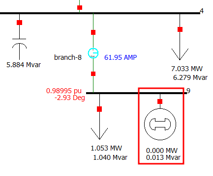
figure 13. Adding a synchronous condenser.
The generator setting should be set to the following:
- MW Output = 0.00
- Available for AGC = unchecked
- Available for AVR = checked
- SetPoint Voltage = V_init = 0.98995 (Initial voltage before adding the generator)
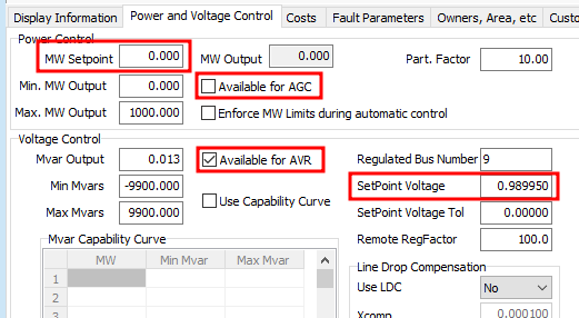
figure 14. Initial synchronous condenser settings.
Solve the case and notice that when the generator is set to the initial voltage it has negligible effect on the system. Record the reactive power consumed by the generator in the appropriate place in the table on the
ECE433 - Lab 3 - Spreadsheet.Change the
Setpoint Voltageof the generator on bus 9 to the per-unit voltage levels listed in the table below for Approach 1. Determine the reactive power consumed by the generator at each voltage setting and record these values in the corresponding table on theECE433 - Lab 3 - Spreadsheet. Note that every time you change theSetPoint Voltageyou need to find the new solution by either clicking on theSolve Power Flow - Newtonbutton or by continuously running the solution by clicking on thePlaybutton in theToolsribbon.
| V (pu) | Q (Mvar) | Q (Mvar ) | V (pu) |
|---|---|---|---|
| V_init: 0.98995 | Q_init: 1.04013 | ||
| 0.9 | 50 | ||
| 0.8 | 100 | ||
| 0.7 | 150 | ||
| 0.65 | 160 | ||
| 0.625 | 170 | ||
| 0.6 | 180 | ||
| 0.575 | 181 | ||
| 0.56 | 182 | BLACKOUT | |
| 0.555 | – | – | |
| 0.55 | BLACKOUT | – | – |
3.6.2 Approach 2
Approach 2
Gradually scale up only the reactive power load on only bus 9 using a similar procedure as in the previous “P-V Curve” sections. As the reactive power load on bus 9 increases the voltage of the bus will decrease. The voltage at the bus and reactive power consumed by the load can then be plotted to produce a Q-V curve.
- Starting again from the base case obtain the Q-V curve using
Approach 2. Adjust the reactive power of the load at bus 9 by either
adjusting it directly or by using the
Scale Casetool as was done before. If you use theScale Casetool make sure to only select bus 9 to scale. Determine the per-unit voltage at bus 9 at each reactive power setting listed in the table in the previous section under Approach 2 and record these values in the corresponding table on theECE433 - Lab 3 - Spreadsheet.
Sign-off
Once you are satisfied that you have collected all of the information required for your lab report get a lab instructor or TA to check your restults and if everything is alright they will sign your sign-off sheet.
3.6.3 Postlab Questions
Q15. Is there any difference between the two Q-V curves created using the 2 different approaches? Explain.
Q16. Why is the initial Setpoint Voltage for the
fictitious condenser used in approach 1 set to the bus voltage of the
original base case?
Q17. Discuss both the advantages and disadvantages of each approach to obtaining a Q-V curve.
4 Postlab
Submit the following on eClass using the
Submit (Lab 3 - Results) link before the postlab due date.
Every student needs to hand-in their own results. Please merge all the
following into a single pdf document in the following order:
Use a scanned/picture copy of the
ECE433 - Lab 3 - Sign-offsheet as your cover sheet coverted to pdf. Make sure your name, student ID, CCID and lab section are visible in the table at the top of the page and make sure that you have obtained the required signatures from your lab instructor or TA during your lab session.A pdf of the completed results tables and plots from the
ECE433 - Lab 3 - Spreadsheet.A pdf of the Answers to the Questions on the
ECE433 - Lab 3 - Postlab Questionssheet.
PDFsam Basic is a free and open source software that can be used for the pdf merge: https://pdfsam.org/download-pdfsam-basic/