Lab 2 - Power Flow Calculations
ECE433 - Power Systems Stability and Transients
Electrical and Computer Engineering - University of Alberta

Figure 1: Power Station
1 Introduction
Power flow (or load flow) characterizes the steady-state operating conditions of a power system. Typical power flow results are bus voltages and branch currents. Power flow calculation is the most fundamental task in power system design and analysis. In this experiment, the power flow of a small industry system will be calculated using a computer program. Sensitivity studies will be performed on the case to demonstrate the steady-state characteristics of power systems. The main objectives are to expose you with the power flow software tools widely used in industry and to gain basic knowledge on how to conduct power flow analysis.
1.1 Summary
Task 1 - Base Case Preparation
Using the values that you prepared for this system at the end of lab 1 build the case in PowerWorld Simulator.
Task 2 - Controlling Bus Voltage with Transformer
Using the base case that you have now prepared use one of the transformers tap ratios to regulate the voltage at a specific bus.
Task 3 - Effect of Capacitor
Resetting your experiment to the base case see how a compensation capacitor effects the system by removing it from the system.
Task 4 - Effect of Load Changes on Bus Voltage
Again resetting your experiment to the base case see how the system is effected by increasing one of the loads. First, you will experiment with how adding real power to the load effects the system and then separately testing to see how adding reactive power effects the system differently.
Task 5 - Load Models
After resetting your experiment to the base case for the last time you will experiment with how either a generator with negative power values or a regular P+jQ load effects the system during steady state.
1.2 Background
1.2.1 The Power Flow Problem
A balanced power system can be modeled as a single-line circuit. It can be characterized by either an admittance matrix \([Y_{bus}]\) or an impedance matrix \([Z_{bus}]\). Almost all modern power flow calculation methods are based on the admittance matrix formulation. The admittance matrices relate bus voltages \([V]\) and bus current injections \([I]\) as follows:
\[[Y_{bus}] [V] = [I] \tag{2.1}\]
Each entry of \([Y_{bus}]\) is \(Y_{ij} = G_{ij} + jB_{ij}\), which could include the admittance data of transmission lines, underground cables, transformers, shunt capacitors and so on. The voltage at bus i can be described in either polar or rectangular coordinates as:
\[V_i = |V_i|∠\delta_i = e_i + jf_i \tag{2.2}\]
The net current injected into the network at bus i in terms of the elements Yij of Ybus is given by the summation
\[I_i = \sum_{j=1}^{N}Y_{ij}V_j \tag{2.3}\]
Let \(P_i\) and \(Q_i\) denote the net real and reactive power entering the network at bus \(i\). Then, the complex conjugate of the power injected at bus \(i\) is
\[P_i-jQ_i=V_i^*I_i=V_i^*\sum_{j=1}^{N}Y_{ij}V_j \tag{2.4}\]
Expanding this equation and equating real and reactive parts, we obtain
\[P_i=\sum_{j=1}^{N}|Y_{ij}V_iV_j|\cos(\theta_{ij}+\delta_j-\delta_i) \tag{2.5}\]
\[Q_i=\sum_{j=1}^{N}|Y_{ij}V_iV_j|\sin(\theta_{ij}+\delta_j-\delta_i) \tag{2.6}\]
Where \(\delta_i\) and \(\delta_j\) are the voltage angles in bus \(i\) and bus \(j\), and \(\theta_{ij}\) is the admittance angle in the branch of \(Y_{ij}\). The above two equations form the basic power-flow equations in the polar coordinate. In power system planning and operation practices, the following data are typically known:
Load demand \(P_i+jQ_i\) at load buses. Since \(P_i+jQ_i\) are known for these buses, they are also called PQ buses.
Real power generation \(P_i\) and scheduled bus voltages \(V_i\) at generator buses. Since \(P_i\) and \(V_i\) are known for these buses, they are also called PV buses.
At least one generator in the system must act as a slack generator whose real power output is adjusted to compensate the real power mismatches (\(P_{generation} - P_{load} - P_{loss}\)) of the entire system. This generator is also used to set a reference angle for the voltages of the system. The bus connecting this generator is therefore called slack (or swing) bus.
The power flow problem is to determine the bus voltages and branch currents under the above given constraints. The equation counted for an N bus network is as follows:
Unknowns to be solved: (\(N-N_{PV}-1\)) magnitudes and (\(N-1\)) phase angles of bus voltages Equations available:
Equations (2.5) and (2.6) for load buses
Equations (2.5) for generator buses
Known voltage magnitude for generator buses
Known voltage magnitude and angle for the slack generator
Since the number of available equations is just equal to the number of unknowns, the load flow problem can be solved.
1.2.2 Newton-Raphson Solution
The power flow equations such as Equations (2.5) and (2.6) are nonlinear equations of the bus voltage magnitudes and angles. They have to be solved employing iterative techniques such as the Newton- Raphson method. The Newton-Raphson method is briefly described here. Let the load flow equation be succinctly rewritten as:
\(y_s = f(x)\)
Where ys is the vector of given constraints such as power injections at load buses, and x is the unknowns that are the bus voltage magnitudes and angles. The procedure of the Newton-Raphson method is:
Newton-Raphson Method
Step 1: Set an initiative starting point \(x_0\).
Step 2: Calculate power mismatch and when \(\Delta x\) gets very small, stop the iteration.
\[\Delta y=y_s−f(x_0)\]
Step 3: Calculate Jacobian matrix at \(x_0\)
\[J=\frac{\partial f(x)}{\partial x}\Biggr\rvert_{x=x(0)}\]
Step 4: Calculate the change vector of \(x\) as
\[\Delta x = J^{−1}\Delta y\]
Step 5: Update the \(x\) vector as
\[x_1 = x_0 + \Delta x\]
Step 6: Use \(x_1\) as a new starting point and go back to Step 1.
1.2.3 Power-flow Studies Procedure
Typical procedures for power flow analysis are as follows:
Collect data of network topology and power system components.
- one-line diagram of the network
- bus voltages
- line and cable impedances (series and shunt data)
- transformer short-circuit data
- data for shunt capacitors and reactors
- supply system fault levels
- bus load data (P and Q)
- generator real power output and scheduled voltage
Organize the data in a form acceptable to the specific power flow program being used.
- rename bus names and numbers
- rename branch names and numbers
- convert the data from real-unit values into per-unit values or from per-unit values into real-unit values
- tabulate the data for documentation
Input the data into the power flow program.
- One typical case is input into the program. This case is called the base case in the experiment.
Run the program on the base case.
- It is quite common that the base case would not run properly at the first time. Debugging of the input data is needed. Two types of situations may happen: 1) the case cannot be solved and 2) the results do not make sense.
- Possible causes of these errors are: 1) network topology error, 2) input impedance error, 3) incorrect bus load or scheduled generator voltages, 4) incorrect transformer settings.
- Some of the methods to identify the causes are: 1) run the power flow on portion of the network (typically starts from the slack bus) and then gradually expand the ‘workable’ portion by including more buses and branches; 2) run power flow with zero or very small loads.
Perform power flow studies.
- Once the quality of base case is confirmed, formal power flow studies can be carried out.
- Typical power flow analysis involves many what-if scenario studies and sensitivity studies.
- A good practice is to save every what-if case (our experiences).
- Finally, the results of scenario studies are compared to help to make engineering decisions.
1.3 Required Software
PowerWorld Simulator
figure 2. PowerWorld Simulator logo.
2 Pre-lab
Please complete the following before attending your scheduled lab session.
2.1 Pre-lab Tasks
Make sure you know where and when to come to the lab by looking at the lab schedule that is available on eClass.
Familiarize yourself with the lab procedures and requirements by reading through the lab manual.
Complete the questions from the ECE433 - Lab 2 - Prelab Questions template. The same questions are shown below.
Have at least, the ECE433 - Lab 2 – Sign-off sheet printed off before coming to the lab.
The ECE433 - Lab 2 - Spreadsheet will be used to record your results for analysis and submission.
Note that there is a ECE433 - Lab2 - Postlab Question template for you to complete as part of your postlab. The same question are shown inline in the lab manual at the appropriate place.
2.2 Pre-lab Questions
What does power-flow or load-flow study refer to?
List the types of the buses that are specified in the formulation of power-flow analysis and explain the characteristics of each bus type.
A 14-bus system has five generator units. List the number of unknown voltage variables to be solved for in a power-flow study.
In power-flow calculations, what are the possible quantities that describe a bus in a power system?
What are the advantages (list two) of using the per-unit system in power-flow analysis?
Can a power-flow study be performed by using the real-unit system to do the power-flow calculations? Explain?
If the reactive power consumption for a load bus is increased, which quantity would be more susceptible to this change; voltage angle or voltage magnitude? Why?
List three methods to increase the voltage of a particular bus in a power system.
3 Lab Procedure
3.1 Base Case Preparation
The system used for this experiment consists of 9 buses and is representative of a medium-sized industrial plant. The system is extracted from a common system that is being used in many of the calculations and examples in the IEEE Color Book series. The plant is fed from a utility supply at 69 kV and the local plant distribution system operates at 13.8 kV. There are 4 transmission lines branches and 4 transformers branches that connect the two generators to all of the different loads throughout the system.
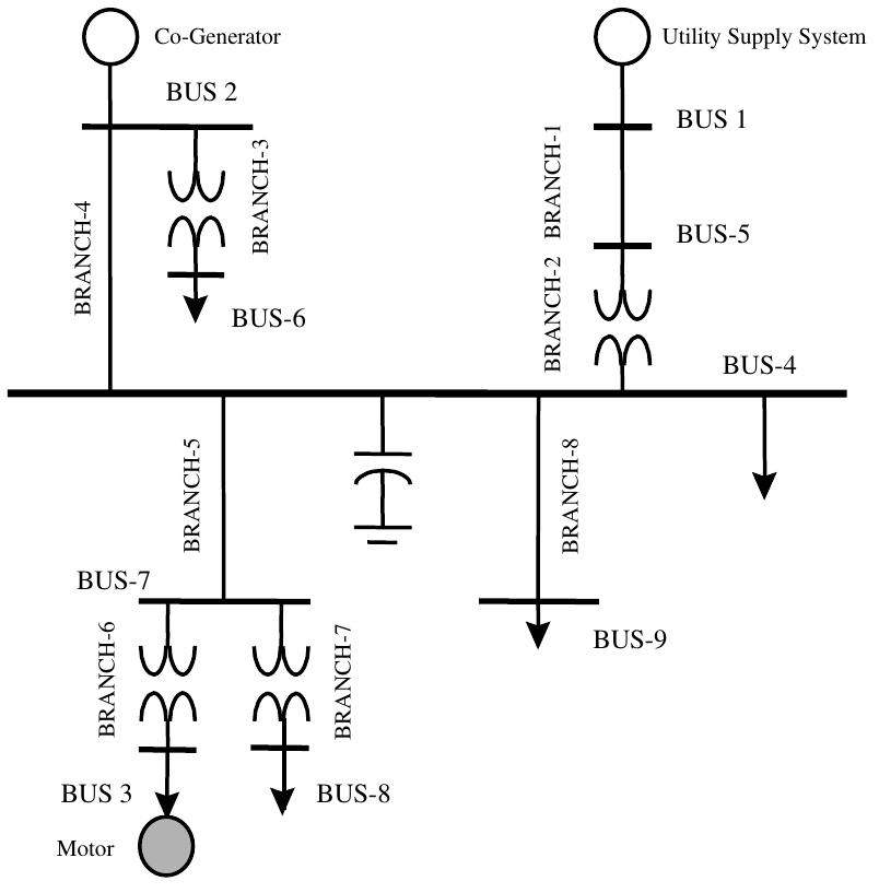
figure 3: A balanced industrial system.
Construct the above industrial system in PowerWorld and enter the parameters that you completed in the postlab for lab 1. Here are the parameters in case you have made mistakes in the preparations. Use a similar procedure to what you did in lab 1 to build the system above.
Once the data have been entered completely, you can solve the power flow. Use the base-case results below to check your system to see if you have entered in everything correctly.
Note
The case may not be solvable at the first run. It is likely that you have to go through a few try-and-error iterations before the case can be set up successfully. So be patient. The key is to make sure all data are entered correctly. In addition to solving the case, you need to check the solution results to verify if the system power flow is reasonable:
Are all voltages close to 1 per-unit?
Is total power generation greater but not too greater than the total load? (the difference between generation and load is system loss)
Are there any branches that have excessive losses?
3.1.1 Base-case Results
To assist you in your case setup the correct results for the case have been provided below. It includes the solved one-line diagram and the bus and branch solutions in the tables below. Your results don’t have to match the correct results exactly in order to be qualified as okay but should be close, talk to an lab instructor or TA if you have any questions. It is best to adjust your one-line diagram so it looks similar to the one below.
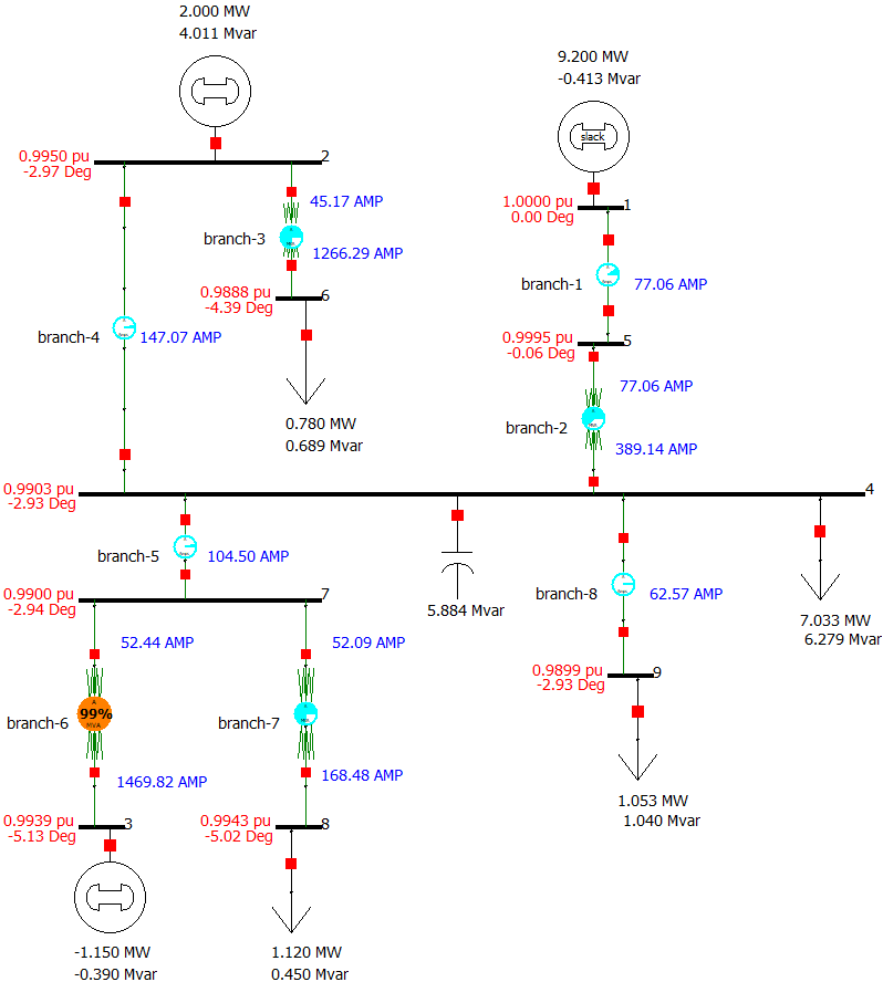
figure 4. Base Case Results
| Bus # | Voltage | Angle | Generation Real Power | Generation Reactive Power |
|---|---|---|---|---|
| per-unit | Degree | MW | MVAR | |
| BUS-1 | 1 | 0 | 9.1999 | -0.4135 |
| BUS-2 | 0.995 | -2.97 | 2 | 4.0109 |
| BUS-3 | 0.99428 | -5.13 | -1.1500 | -0.3900 |
| BUS-4 | 0.99025 | -2.93 | — | — |
| BUS-5 | 0.99954 | -0.06 | — | — |
| BUS-6 | 0.9892 | -4.39 | — | — |
| BUS-7 | 0.99002 | -2.94 | — | — |
| BUS-8 | 0.99465 | -5.02 | — | — |
| BUS-9 | 0.98995 | -2.93 | — | — |
| Branch # | Current at from bus | Current at to bus | Real Power Loss | Reactive Power Loss |
|---|---|---|---|---|
| Amp. | Amp. | MW | MVAR | |
| branch-1 | 77.06 | 77.06 | 0.004715 | 0.010041 |
| branch-2 | 77.06 | 389.14 | 0.027096 | 0.460609 |
| branch-3 | 45.17 | 1265.79 | 0.007083 | 0.041858 |
| branch-4 | 147.07 | 147.07 | 0.007538 | 0.015015 |
| branch-5 | 104.5 | 104.5 | 0.000468 | 0.000393 |
| branch-6 | 52.43 | 1410.48 | 0.008831 | 0.052985 |
| branch-7 | 52.09 | 166.81 | 0.006353 | 0.050822 |
| branch-8 | 62.57 | 62.57 | 0.000351 | 0.000293 |
Warning
Once you have a working base case, save it somewhere to archive it in
case you break the case at some point during the laboratory. Do not
forget to make sure that both the .pwb and
.pwd are saved.
Sign-off
- Once you are satisfied with your base case construction get a lab instructor or TA to check your system and if everything is alright they will sign your sign-off sheet.
3.1.2 Postlab Questions
Note
All of the questions are both posted inline in the lab manual so you
can consider possible answers while working on the lab. The questions
are intended to be answered as a postlab exercise on the provided
ECE433 - Lab 2 - Postlab Questions template.
- For each branch in the system are the ‘from bus’ and ‘to bus’ currents equal? In which cases are they equal and in which cases are they different? Explain why.
3.2 Controlling Bus Voltage with Transformer
Note
In the following sections:
- Controlling Bus Voltage with Transformer
- Effect of Capacitor
- Effect of Load Changes on Bus Voltage
- Load Models
Start with the base case then make the appropriate changes to obtain
the required result. Make sure that you re-run the case after the
changes have been made. Once you are satisfied with the results it is a
good idea to save the new case as a separate file with a new
descriptive. Use the Model Explorer to save the
Buses and Branches State tables in a similar
manner that you did in lab 1 for use to complete the
ECE433 - Lab 2 - Spreadsheet. In most sections we are
comparing the new case to the base case to determine what the effect of
the change was.
One of the methods to control the voltage of a load bus is through adjusting the tap-ratio of its feeding transformer. Use PowerWorld Simulator to demonstrate that you are able to accomplish this.
- Adjust the
Off-nominal Tap Ratioof theBranch-3transformer in order to get 0.98 pu (+/- 0.1%) voltage onBus-6. Make sure to re-run the case to update the results. Save the results as required. Make sure to note theOff-nominal Tap Ratiothat was used. Record your final results in theECE433 - Lab 2 - Spreadsheet.
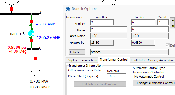
figure 5. Changing the Off-nominal Turns Ratio.
3.2.1 Postlab Questions
- In the case that a bus does not have a private feeding transformer (e.g. bus 9), so changing the transformers tap ratio is not possible, is there another way to adjust the voltage of the bus?
3.3 Effect of Capacitor
Reactive power compensation capacitors are used to reduce the amount
of current in branches to lower overall losses in the system. Use
PowerWorld Simulator to demonstrate this by comparing the base case
which has a shunt capacitor bank on Bus-4 to a new case
with the shunt capacitor turned off.
- Making sure to start from the base case, turn off the shunt reactive
power compensation capacitor at
Bus-4by opening the breaker as shown below. Make sure to re-run the case to update the results. Save the results as required. Record your final results in theECE433 - Lab 2 - Spreadsheet.
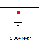
figure 6. Shunt compensation capacitor connected to circuit.
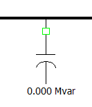
figure 7. Shunt compensation capacitor disconnected from circuit.
3.3.1 Postlab Questions
In power-flow analysis is a capacitor a reactive power source or sink?
What are the most noticeable changes in the system that are caused by switching off the compensation capacitor? Explain your observations.
3.4 Effect of Load Changes on Bus Voltage
The amount (magnitude) and type (real or reactive) of load will effect the systems buses differently. Use PowerWorld Simulator to demonstrate in 2 different cases how different types of loads effect the buses. First, increase the real power at one of the buses to see the effect on the system relative to the base case and secondly increase the reactive power so the differences can be determined.
Making sure to start from the base case, scale the real power (P) at
Bus-3by 50% by adjusting theMW Outputof theGenerator(which is acting like a motor) connected toBus-3. Make sure to re-run the case to update the results. Save the results as required. Record your final results in theECE433 - Lab 2 - Spreadsheet.Making sure to start from the base case again, now scale the reactive power (Q) at
Bus-3by 50% by adjusting theMvar Outputof theGenerator(which is acting like a motor) connected toBus-3.. Make sure to re-run the case to update the results. Save the results as required. Record your final results in theECE433 - Lab 2 - Spreadsheet.
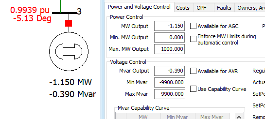
figure 8. Changing the P and Q load magnitude by 50% on bus 3.
3.4.1 Postlab Questions
What is the most significant change caused by a 50% real power load increase at one of the buses?
What is the most significant change caused by a 50% reactive power load increase at one of the buses?
Explain in your own words why the answers to the 2 previous questions are not the same.
3.5 Load Models
The Generator (being used as a motor load) at
Bus-3 is modeled as a machine in the base case. The model
for machines is a voltage source behind its transient or sub-transient
impedances. The voltage source is adjusted by the load flow program to
produce a load level specified in the input data. For load flow studies,
a motor could also be modeled using a regular load model (constant
P+jQ). Use PowerWorld Simulator to determine if there is any difference
on load flow results caused the two load models.
- Making sure to start from the base case, replace the machine model
at
Bus-3with a regular P+jQ load using the same P and Q input data. Make sure to re-run the case to update the results. Save the results as required. Record your final results in theECE433 - Lab 2 - Spreadsheet.
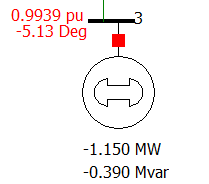
figure 9. The motor on bus 3 from the base case.
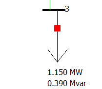
figure 10. The new load connected at bus 3.
3.5.1 Postlab Questions
- Are there any major differences between the power-flow results when a P+jQ load is used instead of a generator on the same bus? Explain your observations.
Sign-off
- Once you are satisfied that you have collected all of the results required to complete the postlab get a lab instructor or TA to check what you have and if everything is alright they will sign your sign-off sheet.
4 Postlab
Submit the following on eClass using the
Submit (Lab 2 - Results) link before the postlab due date.
Every student needs to hand-in their own results. Please merge all the
following into a single pdf document in the following order:
Use a scanned/picture copy of the
ECE433 - Lab 2 - Sign-offsheet as your cover sheet coverted to pdf. Make sure your name, student ID, CCID and lab section are visible in the table at the top of the page and make sure that you have obtained the required signatures from your lab instructor or TA during your lab session.A pdf of the completed results tables and plots from the
ECE433 - Lab 2 - Spreadsheet.A pdf of the Answers to the Questions on the
ECE433 - Lab 2 - Postlab Questionssheet.
PDFsam Basic is a free and open source software that can be used for the pdf merge: https://pdfsam.org/download-pdfsam-basic/