Figure 1: Transmission Tower

1 Introduction

This laboratory exercise serves as an introduction to one of many software programs that are used for electric power systems. This simulation program, PowerWorld Simulator, will be used for the first three labs of this course.

Below is a summary of what you will be working on during this first laboratory.

1.1 Summary

Task 1 - Run a Sample Case

Open an existing sample case to demonstrate the programs user interface, how to run a case, and how to see the results.

Task 2 - Build a New Case

Create a simple case from scratch to demonstrate how to place commonly used components in power system and how to configure them.

Task 3 - Results

Run the case that you created in task 2 to collect results to submit as part of your lab report.

1.2 Required Software

PowerWorld Simulator is a program designed to give students and/or engineers intuitive insight into power system operations. It accompanies the textbook “Power System Analysis and Design” by J. Glover and M. Sarma. The latest Education version of the software can be downloaded from the PowerWorld’s website.

figure 2. PowerWorld Simulator logo.

https://www.powerworld.com/download-purchase/demo-software

This appendix provides a brief introduction to the PowerWorld Simulator V.19 and helps you to get started with the software. You are encouraged to read the software’s help files and experience the features of the program by yourself.

https://www.powerworld.com/download-purchase/download-help-files

This simulator is an interactive power system simulation package designed to simulate high voltage power system operation. It is mainly used for basic and intermediate power system analysis. In terms of technical characteristics, power system analyses can be classified into three levels:

Basic power system analyses such as power flow calculation and fault analysis
Intermediate power system analyses such as harmonic analysis, motor starting, and stability
Advanced power system analyses such as electromagnetic transients analysis (EMTP)

2 Pre-lab

For the first lab there is nothing to hand-in as a Pre-lab but please come to the lab prepared by doing the following.

2.1 Pre-lab Tasks

Make sure you know when to come to the lab by looking at the lab schedule that is available on eClass.
Familiarize yourself with the lab procedures and requirements by reading through the lab manual.
Have at least, the ECE433 - Lab 1 – Sign-off sheet printed off before coming to the lab.
If you would like to use pen and paper to record your results you could also print off the ECE433 - Lab 1 - Results sheet.

3 Lab Procedure

3.1 Run a Sample Case

Launch PowerWorld Simulator and open a sample case.
1. Launch PowerWorld Simulator in Windows by using the start menu.
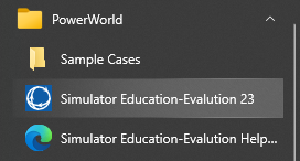
figure 3. PowerWorld program launcher.
1. From the File menu Select Open Case... and select the B7flatlp.pwb case in the Sample cases directory located at C:\Users\Public\Documents\PowerWorld\23\Sample Cases.

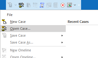
figure 4. Open case dialog.

The following sample case is then loaded into PowerWorld Simulator. We will use this sample case to familiarize ourselves with a few features of this software package.

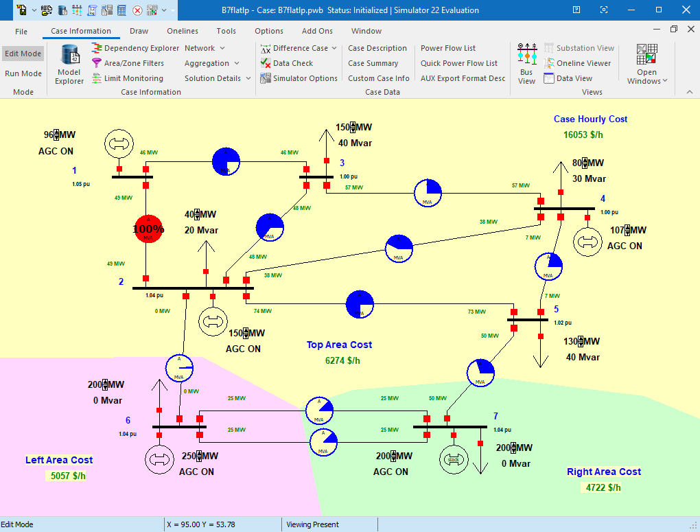
figure 5. The sample case.

3.1.1 PowerWorld User Interface

PowerWorld’s user interface consists of a ribbon across the top of the program. Important terminology regarding the ribbon is depicted in the image below.

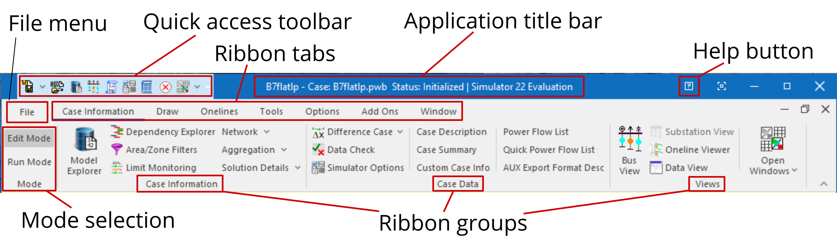
figure 6. The ribbon in PowerWorld Simulator.

The entire strip across the top is called the ribbon and contains all of the tools that are used. The ribbon consists of several ribbon tabs which are organized into groups. The 7 ribbons that make up the toolbar are summarized below.

Table 1. The ribbon tabs available on the toolbar.
Ribbon	Description
Case Information	primarily used to navigate and look through all the data in your model.
Draw	primarily used to draw new oneline diagrams or edit existing onelines by adding, moving, formatting, or resizing existing oneline objects. Most of the options on the Draw ribbon tab are only available in Edit Mode.
Onelines	primarily used after you have already created a oneline diagram. This ribbon provides features for customizing the appearance of your oneline diagram.
Tools	this ribbon provides access to all of the analysis tools that are available in the base package of PowerWorld Simulator. You will use this ribbon when you are performing power flow analysis, contingency analysis, or using the sensitivities tools for instance.
Options	all of the buttons on this ribbon are also available on one of the other ribbons, however this ribbon brings all the options in the software into one place.
Add Ons	this ribbon provides access to all the add-on tools available for Simulator including the OPF, SCOPF, ATC, and PVQV tools. If you have not purchased these tools then the options will be grayed out.
Window	this ribbon provides access to customizing the Windows in the User Interface. It also has some information reading help topics.

It is important to note that PowerWorld Simulator has two modes of operation, Edit Mode and Run Mode. The Mode ribbon group is placed in the left side of top ribbon and is always visible.

Table 2. The two modes, Edit and Run.
Mode	Description
Edit Mode	Switches the program to Edit Mode, which can be used to build a new case or to modify an existing one.
Run Mode	Switches the program to Run Mode, which can be used to perform a single Power Flow Solution or a timed simulation with animation.

3.1.2 Solve the case

Run the case by doing the following.
1. Switch to Run Mode.
2. On the Tools ribbon, push the Play button from the Power Flow Tools ribbon group.
3. The case is then solved and becomes interactive. For example you can adjust the power supplied to the system by the generators or the power consumed by the loads by using the up and down arrows next to each of the devices power display. You can also disconnect loads, generators or branches by using the red squares that connect them to a bus.

3.1.3 Inspect results

Some of the results can be observed directly on the one-line diagram. For example, the voltages are listed beside the buses, the real and reactive power output of the generators is shown next to the corresponding generator, the power flow is indicated along the branches, etc.

Output results can also be obtained after the applicable case has been run.

From the Case Information ribbon click on the Network menu and select Buses to view the related bus information in a table format. You can access tables for generators, loads and branches in a similar manner as above.

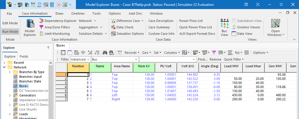
figure 7. Bus records.

3.1.4 Edit input data

You can edit the input data of each component in the one-line diagram by doing the following.
1. Switch to Edit Mode.
2. Right-click on any component (ie. generator, load, branch, bus, etc…) in the one-line diagram and select its Information Dialog... (Generator shown below).
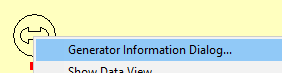
figure 8. Right clicking on component
1. A options dialog box appears (Generator Options shown below) which allows you to configure the component.
2. You can then change the configurations as required.

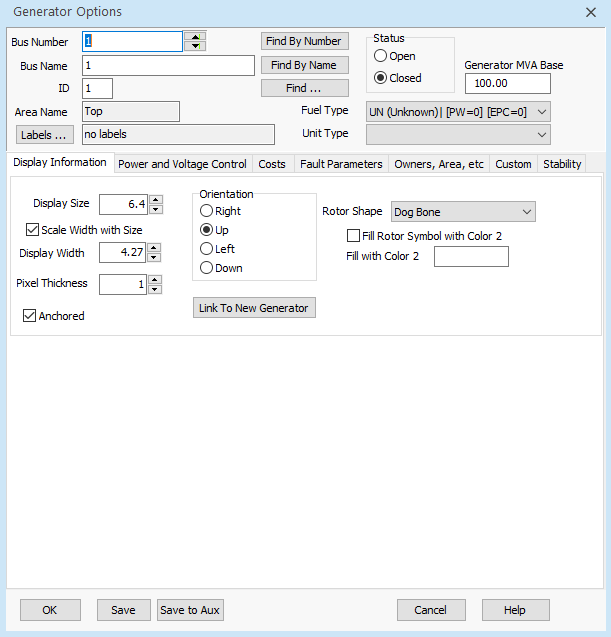
figure 9. Generator options.

3.2 Build a New Case

A simple case consisting of 3 buses can be created easily using PowerWorld Simulator. Bus 1 is connected to the utility (Source), Bus 2 is connected to the generator (Gen) and Bus 3 provides power to the load (Load). One transmission line (from Bus 2 to 3) and one transformer (from Bus 1 to 3) build up the network. A switched shunt capacitor is connected to Bus 3 which is available to boost the bus voltage if required.

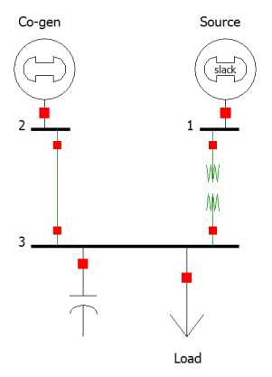
figure 10. Screenshot of the new case in PowerWorld Simulator.

Start a new simulation by clicking on File and then New Case and make sure that you are currently in Edit Mode. You will always need to be in Edit Mode in order to insert or edit any component.

3.2.1 Insert Buses

Create Bus 1 for your simulation.
1. Select the Draw ribbon and under the Individual Insert ribbon group select Network\Bus. Insert the Bus into the one-line diagram by clicking on the canvas to place the bus in your desired position.
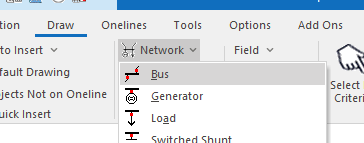
figure 11. Bus options for Bus 1.
1. A dialog box named Bus Options will appear.
Configure Bus 1 by entering the following information.
1. The Bus must have a unique Bus Number (= 1), a Bus Name (= Source) and Nominal Voltage (= 69kV).
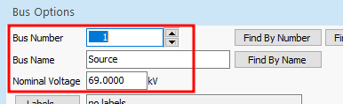
figure 12. Bus options for Bus 1.
1. Under the Bus Information tab we can set the Bus Voltage in p.u. (= 1.00) and the voltages Angle in degrees (= 0).
2. We want Bus 1 to be the systems slack bus, so make sure the System Slack Bus box is checked.
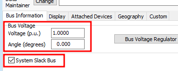
figure 13. Bus options for Bus 1.
Click Save and then OK to finish Bus 1.
Create Buses 2 and 3 similarly.
1. Give Bus 2 a Bus Name of Co-Gen and Nominal Voltage of 13.8kV. This bus will be a PV-bus and be connected to a co-generator, therefore a Bus Voltage in p.u. is required. Enter 0.995 in the corresponding box. There is no need to enter an Bus Voltage Angle so leave it empty.
2. Give Bus 3 a Bus Name of Load and a Nominal Voltage of 13.8kV. This bus will be a typical PQ-bus and have a load connected to it. Neither a Bus Voltage or Angle setting is needed so leave them as they are.

3.2.2 Add Generators

The utility supply system is represented as a generator with unlimited capacity. In this example, we will learn how to use PowerWorld Simulator to model this component.

Create a utility supply using a generator on Bus 1.
1. Select the Draw ribbon and under the Individual Insert ribbon group select Network\Generator. Insert the Generator into one-line diagram by clicking on Bus 1 (Source) to attach the Generator to it.
2. A dialog box named Generator Options will appear.
Configure the utility generator by entering the following information.
1. Note that the Bus Number is set to 1 and the Bus Name is set Source. Also note that the Gernerator MVA Base value is set to 100.
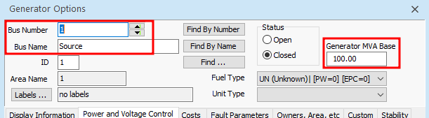
figure 14. Bus 1 generator options (Display Information).
1. In the Power and Voltage Control tab make sure the following options are as listed below.
  - MW Setpoint = 0.
  - Available for AGC = unchecked.
  - Enforce MW limits = unchecked.
  - Available for AVR = checked.
  - SetPoint Voltage = 1.00 p.u.
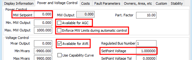
figure 15. Bus 1 generator options (Power and Voltage Control).
1. After setting up the generator we would also like to change the way it is displayed on the one-line by going to the Display Information tab. Make the following changes as shown below.
  - Display Size = 7
  - Orientation = Up
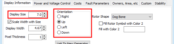
figure 16. Bus 1 generator options (Display Information).
Click Save and then OK to finish adding the generator to Bus 1 as the utility supply.
Add a second generator, this time on Bus 2, in a similar manner that was done above using the following information. This generator is an actual generator that is used on the local system.
- Connected to Bus 2
- MW Setpoint = 2.
- Mvar Output will be calculated and filled in by the program.
- Available for AGC = checked.
- Enforce MW limits = unchecked.
- Available for AVR = checked.
- SetPoint Voltage = 0.995 p.u.
- Display Size = 7
- Orientation = Up

3.2.3 Add a Load

Add a load to the system by doing the following.
1. Select the Draw ribbon and under the Individual Insert ribbon group select Network\Load. Insert the Load into one-line diagram by clicking on Bus 3 (Load) to attach a load to it.
2. A dialog box named Load Options will appear.
Configure the load by entering the following information.
1. Note that the Bus Number is set to 3 and the Bus Name is set Load.
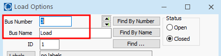
figure 17. Bus 3 load options
1. In the Load Information tab make sure the following options are as listed below.
  - Under Constant Power set the MW Value to 7.00 and the Mvar Value to 6.30.
  - Under the same Constant Power tab under Display Information make sure that the Display Size is set to 7.00 and the Orientation is set to Down.
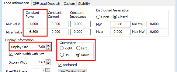
figure 18. Bus 3 Load Information options
Click Save and then OK to finish adding the load to Bus 3.

3.2.4 Add a Shunt Capacitor

Add a shunt capacitor to the system by doing the following.
1. Select the Draw ribbon and under the Individual Insert ribbon group select Network\Switched Shunt. Insert the shunt capacitor into one-line diagram by clicking on Bus 3 (Load) to attach it to the same bus as the load.
2. A dialog box named Switch Shunt Options will appear.
Configure the shunt capacitor by entering the following information.
1. Note that the Bus Number is set to 3 and the Bus Name is set to Load.
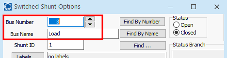
figure 19. Bus 3 switched shunt options
1. Under the Parameters tab set the Nominal Mvar to 6 and the Control Mode to Fixed.
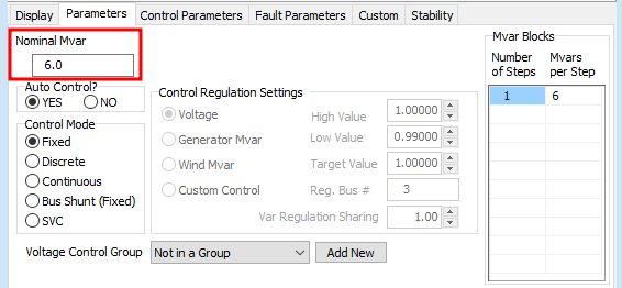
figure 20. Switched shunt parameters
1. Under the Display tab set the Display Size to 7.0 and the Orientation to Down.
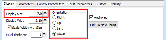
figure 21. Switched shunt parameters
Click Save and then OK to finish adding the shunt capacitor to Bus 3.

3.2.5 Add a Transmission line

Buses in a power system are usually connected together by branches which are most commonly either a transmission lines or a transformer.

Add a transmission line to the system between buses 2 and 3 by doing the following.
1. Select the Draw ribbon and under the Individual Insert ribbon group select Network\Transmission Line. Insert the transmission line into one-line diagram by first clicking on Bus 2 to start the transmission line and then double clicking on Bus 3 to finish it.
2. A dialog box named Branch Options will appear.
Configure the transmission line by entering the following information.
1. Note that the From Bus Number is set to 2 and that the To Bus Number is set to 3.
figure 22.
1. Under the Parameters tab set the Per-Unit Impedance Parameters and MVA Limits as follows.
  - Series Resistance (R) = 0.06
  - Series Reactance (X) = 0.12
  - Leave both Shunt parameters = 0.00.
  - Limit A = 10.0
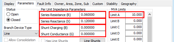
figure 23.
Click Save and then OK to finish adding a transmission line to connect Buses 2 and 3.

3.2.6 Add a Transformer

Buses in a power system are usually connected together by branches which are most commonly either a transmission lines or a transformer.

Add a transformer to the system between buses 1 and 3 by doing the following.
1. Select the Draw ribbon and under the Individual Insert ribbon group select Network\Transformer. Insert the transformer into one-line diagram by first clicking on Bus 1 to start the transformer and then double clicking on Bus 3 to finish it.
2. A dialog box named Branch Options will appear.
Configure the transformer by entering the following information.
1. Note that the From Bus Number is set to 1 and that the To Bus Number is set to 3.
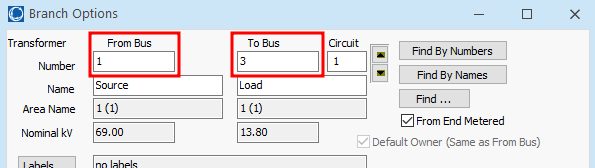
figure 24.
1. Under the Parameters tab set the Per-Unit Impedance Parameters and MVA Limits as follows.
  - Series Resistance (R) = 0.03
  - Series Reactance (X) = 0.53
  - Shunt and Magnetizing parameters = 0.00.
  - Limit A = 10.0
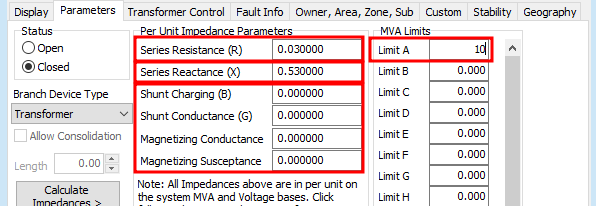
figure 25.
1. Under the Transformer Control tab set the Transformer Information as follows.
  - Off-nominal Turns Ratio = 1.01
  - Phase Shift (degrees) = 0.00
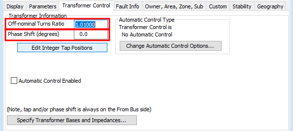
figure 26.
Click Save and then OK to finish adding a transformer to connect Buses 1 and 3.
Run the case that you have created by switching to Run Mode and clicking on the Play button in the Tools Ribbon. Make sure it is working by inspecting the results as describe in “Run a Sample Case” section of the lab manual. Adjust anything if necessary.

3.2.7 Editing Display Information

You can edit the displayed information on the one-line diagram by adding or removing the information that you desire.

For example, you can display the p.u. bus voltage of any bus in the system by doing the following.
1. Make sure you are in Edit Mode and right click on a bus that you wish to see the data on and select ‘Add New Fields Around Bus’.
2. A dialog box appears named Insert New Fields around selected objects asking you to choose the position of the new field. Choose the position as you wish.
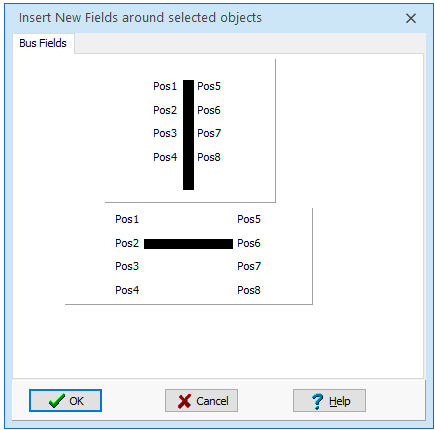
figure 27. Add position for new field to display on One-line.
1. A new dialog box named Bus Field Options appears. From the Type of Field area at the bottom select Bus Voltage (p.u.). Choose 4 for Digits to Right of Decimal. The p.u. bus voltage then displays in the oneline diagram.
2. You can then remove any display information by simply selecting it and hitting the Delete key.

Similarly to above, you can display information for generators, loads, shunt capacitors, transmission lines and transformers. Once the case is solved the load flow results will be displayed on the one-line diagram as demonstrated below.

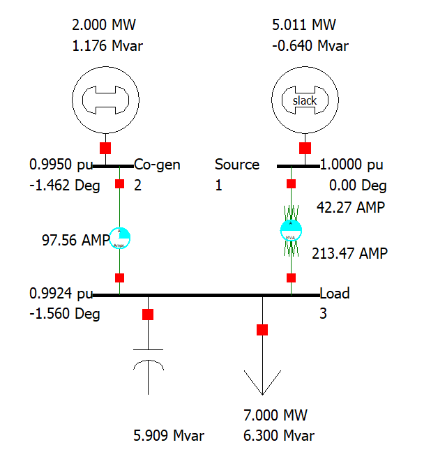
figure 28. Completed One-line diagram.

3.2.8 Save the Case

Save the case by doing the following.
1. Under the file menu click on Save Case As... to save the Case and Oneline diagram that you have created.
2. Click on Save once you have found an appropriate place to save your case and have given it an appropriate name.
3. PowerWorld Simulator will then open up a Add a comment dialog which allows you to make some notes on the case that you are saving. Hitting either Add or Skip will then save your case.
4. Note that PowerWorld will then save the following 2 files, you will need both if you want reopen your case.
  - .pwb = Contains the Case information.
  - .pwd = Contains the Oneline diagram.
5. It is also important to note that if you modify a saved case, make sure to save changes in both the .pwb and .pwd files by using Save Case and Save Oneline, respectively.
Demonstrate the working case that you have constructed for a Lab Instructor or TA and obtain the required signature on the Sign-off sheet.

3.3 Results

Once you are confident that you have entered and run the case correctly you need to collect the results by doing the following.
1. While in either Edit Mode or Run Mode from the “Case Information” ribbon select Network/Buses.... The table containing the bus records will appear in the Model Explorer. The other required tables listed below can also be opened in a similar manner, or alternatively, by selecting the appropriate table in the Model Explorer.
  - Generators
  - Loads
  - Branch Input (Line and Transformer)
  - Branch State (Line and Transformer)
  - Switched Shunts
2. You can either copy the values directly from the Model Explorer to the “Results sheet” or save the tables by right clicking on the table you want to save and selecting Save As/CSV (Comma delimited...)/Column Headers and saving it somewhere appropriate. These files can then be viewed in a spreadsheet program after the lab and need to be inserted into the Results sheet for submission. When recording results in the Results sheet make sure to include values to at least three decimal places. Note that not all values in the PowerWorld Simulator tables are required in the Results tables.
Once all of the records have been recorded get an Lab Instructor or TA to look at them and sign-off in the appropriate place on your Sign-off sheet.

4 Postlab

Submit the following on eClass using the Submit (Lab 1 - Results) link before the postlab due date. Every student needs to hand-in their own results. Please merge all the following into a single pdf document in the following order:

Use the completed Lab Sign-off sheet as your cover sheet. Make sure your name, student ID, CCID and lab section are visible at the top of the page and make sure that you have obtained the required signatures.
The Answers to the Questions on the Results sheet.
The Results tables from the Results sheet.
The Data preparation for Lab 2 tables located on the Results sheet. Described in the ‘Appendix’ section.

PDFsam Basic is a free and open source software that can be used for the pdf merge: https://pdfsam.org/download-pdfsam-basic/

4.1 Appendix - Lab 2: System Description

For lab 2 we will using the case described in the following one-line diagram and tables below. The case consists of 9 buses and is representative of a medium-sized industrial plant. The system is extracted from the IEEE Color Book series.

The industrial plant is connected to the utility supply of 69.00 kV at BUS-5 and then is distributed throughout the plant at voltages of 13.80 kV or lower. Capacitance of the overhead lines and cables are neglected.

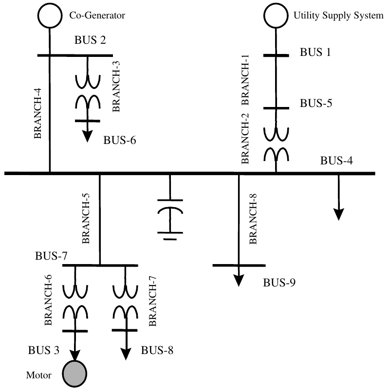
figure 29: A balanced industrial system.

4.1.1 Data Preparation

Use the instructions below to fill out the ‘Data Preparation for Lab 2’ tables located on the Results sheet. The problem is that the data given in the IEEE Color Book series needs to be prepared properly so the data can be entered into PowerWorld Simulator in the format that it expects. It is important that you prepare these tables as accurately and clearly as possible so lab 2 can run smoothly.

Table 1. Line & Cable Branch Preparation
1. From the tables below figure out what the rated voltage of each Line branch is.
2. From the Per-Unit Line and Cable Impedance Data table below re-calculate new per-unit values that will be entered into PowerWorld Simulator while using a \(S_{BASE}\) of 100 MVA. Note that all the of the per-unit values in the table below are calculated with a \(V_{BASE}\) of 13.8 kV regardless of the nominal voltage of the branch.
Table 2. Transformer Branch Preparation
1. From the Transformer Data table below determine the rated kVA of each transformer as well as each transformers rated primary and secondary voltages.
2. Determine each transformers tap setting as an off-nominal turns ratio from the Transformers Data table.
3. Re-calculate new per-unit values from the Transformer Data table that will be entered into PowerWorld Simulator while using a \(S_{BASE}\) of 100 MVA. Note that all the of the per-unit values in the table below are calculated with a \(V_{BASE}\) and \(S_{BASE}\) of the transformers voltage and power ratings, respectivily.
Table 3. Shunt Capacitor Susceptance
1. Calculate the shunt capacitors susceptance per phase.
Table 4. Load Information
1. Obtain the load information from the `Generation, Load, and Bus Voltage Data.
Table 5. Generator and Motor Information
1. There are 3 generators used in this example case. One of the generators is used with negative numbers to act like a motor load. Determine which type of bus each of the 3 generators are connected to, a slack, PV or PQ bus.
2. Knowing which type of bus each one is determine the required known parameters for each bus.

4.1.2 Data Tables

Table 1
Per-Unit Line and Cable Impedance Data (\(V_{BASE} = 13.8 kV, S_{BASE} = 10,000 kVA)\)
branch #	From	To	R (pu)	X (pu)
branch-1	BUS-1	BUS-5	0.01390	0.02960
branch-4	BUS-2	BUS-4	0.00610	0.01215
branch-5	BUS-4	BUS-7	0.00075	0.00063
branch-8	BUS-4	BUS-9	0.00157	0.00131

Table 2
Transformer Data
Branch #	From	To	Voltage	Tap	kVA	%R (pu)	%X (pu)	HV	LV
branch-2	BUS-5	BUS-4	69:13.8	69.69	15000	0.4698	7.9862	Yg	Yg
branch-3	BUS-2	BUS-6	13.8:0.48	13.45	1500	0.9593	5.6694	Yg	Yg
branch-6	BUS-7	BUS-3	13.8:0.48	13.45	1250	0.7398	4.4388	Yg	Yg
branch-7	BUS-7	BUS-8	13.8:4.16	13.45	1725	0.7442	5.9537	Yg	Yg

Table 3
Generation, Load, and Bus Voltage Data
Bus	V (p.u.)	P_Gen (kW)	Q_Gen (kVar)	P_Load (kW)	Q_Load (kVar)
BUS-1	1.000
BUS-2	0.995	2000
BUS-3				1150.00	390.00
BUS-4				7032.87	6279.00
BUS-5
BUS-6				780.00	689.13
BUS-7
BUS-8				1119.74	450.00
BUS-9				1053.00	1040.13

Table 4
Motor and Co-Generator Data
Item	Motor (BUS-3)	Generator (BUS-2)
Size	1200 kVA	3000 kVA
Sub-transient R	0.010 pu	0.002 pu
Sub-transient X	0.200 pu	0.112 pu
Connection	Delta	Yg

4.1.3 Additional Information

Additional data needed to conduct power flow and fault analyses for the example industrial system include the following:

Supply power system equivalent impedance. The utility supply system has a three-phase fault level of 1000 MVA and X/R ratio of 22.2. It has a single-phase fault level of 250MVA and X/R ratio of 18.2.
The correction capacitors of plant power factor are rated at 6 MVar. As is typically done, leakage and series resistance of the bank are neglected in this study.
All loads are shown as 3 phase values.

Lab 1 - Intro to PowerWorld Simulator

ECE433 - Power Systems Stability and Transients

Electrical and Computer Engineering - University of Alberta