2.1 Background

• AC Waveforms
• Average
• RMS
• Phase
• AC Resistors
• Capacitors
• Non-ideal Capacitors
• Inductors
• Non-ideal Inductors
• Series Resistor Capacitor Circuits
• Series Resistor Inductor Circuits
• XYZ’s of Oscilloscopes
• XYZ’s of Function Generators

2.2 Equipment List

• Student Printed Circuit Board
• BNC & Banana Cables
• Digital Multimeter
• Oscilloscope
• Function Generator

3.1 Equipment Familiarization

3.1.1 The Oscilloscope

The oscilloscope or “scope” is one of the most versatile and heavily used electronic measuring instruments in science, engineering, and industry. The oscilloscope earns its status as an important instrument because it neatly graphs how voltage varies as a function of time. Time varying voltage signals are not only important in electronic devices but also useful in measuring all kinds of other types of signals that are converted into an electrical signal by a transducer. A transducer is a device that converts one type of energy to another.

figure 1. Tektronix TDS 1002 Oscilloscope

1. Getting started with the oscilloscope.

   1. Turn the oscilloscope on by pressing the main power switch on the top of the device.

   2. The oscilloscope probe is used to connect voltage signal sources to the oscilloscope. These probes have a selector switch on them to adjust their attenuation factor (x1/x10). On the side of the probe select the x10 option.

   

   figure 2. Typical oscilloscope voltage probe

   3. Connect one end of the oscillscope probe to the ‘CH1’ BNC input and connect the other end of the probe to the ‘PROBE COMP’ input as shown in the picture below. Make sure the ground lead (the alligator clip) of the probe connects to the terminal marked ground of the ‘PROBE COMP’.
   

   figure 3. Oscilloscope probe comp setup

   4. On the ocsilloscope locate and press the ‘DEFAULT SETUP’ button which puts the oscilloscope in a standard default state. Then locate and press the ‘AUTOSET’ button which will try and configure the oscilloscope settings so that an appropriate waveform for the incoming voltage connected to ‘CH1’ is displayed appropriately on the display as shown below. The ‘PROBE COMP’ output that we’ve connected to provides a test signal for the oscilloscope that is a 1 kHz squarewave that jumps from 0V to 5V.
   

   figure 4. Oscilloscope probe comp test waveform

   5. We will now use this ‘PROBE COMP’ signal to explore the 3 main sections of the oscilloscope controls: Vertical, Horizontal and Trigger.

3.1.1.1 Vertical Section

The vertical section controls the y-axis of the displayed incoming voltage signal. There is one set of controls for every input channel. In our case since this is a 2-channel oscilloscope there are 2 sets of controls. The vertical controls are ‘POSITION’, ‘VOLTS/DIV’ and ‘CH 1/2 MENU’ which all contribute to how the incoming waveform is displayed on the vertical/y-axis.

figure 5. Vertical section controls

The key points about the vertical/y-axis are:

• It is the voltage axis. The higher the incoming voltage, the farther from the ‘ground’ (0 Volt level) the graph moves for a given ‘VOLTS/DIV’ setting.
• Voltage can be positive or negative relative to ‘ground’. Positive input voltages moves the graph point above the ‘ground’; negative input voltage moves it below the ‘ground’.

Vertical Position

Each input channel has a ‘ground’ (0 Volt level) indicator on the left edge of the screen. Below is an image showing the vertical position of channel 1 which should now be in the vertical center of the display.

figure 6. Vertical position indicator

The ‘POSITION’ control will move this position indicator up and down on the display which in turn will also move the incoming voltage waveform up and down on the display.

Volts per Division

A typical oscilloscope will have 8 vertical divisions on the display. You can change the graph’s y-axis scale (expressed in volts per division or VOLTS/DIV) using the VOLTS/DIV knob to control how the incoming voltage waveform is scaled when it is displayed on the graph. It doesn’t change the value of the input voltage. In the bottom left hand corner you can see what the current setting for the volts per division, as shown in the image below.

figure 7. Voltage per division indicator

The displayed waveform should currently span approximately 2.5 vertical divisions of the oscillscope’s screen and the volts per division is currently set for 2.00V. When you multiply those 2 numbers together you get 5V. Which is the approximate value of the ‘PROBE COMP’ signal.

Ch 1 Menu

The vertical menu has the following options. The defaults are in bold and are typical settings.

• Coupling - (DC/AC/Ground)
  DC coupling will show the waveform as is, AC coupling will filter/remove the DC component, and Ground coupling disables the input and shows the 0V level.
• BW Limit - (Off = 60Mhz/On = 20Mhz)
  This adds a filter to the inputs before it is displayed on the screen effectively limiting the bandwidth.
• Volts/Div - (Course/Fine)
  Course allows you to go through the normal Volts/Div settings where as Fine allows you to adjust the Volts/Div at very small steps.
• Probe - (1X/10X/100X/1000X)
  This setting should match the probe that you are currently using so the values on the scope display properly.
• Invert - (Off/On)
  Simply inverts the displayed waveform. Would be the same as reversing/swapping the probe connections.

2. Adjust the following ‘CH 1’ ‘VERTICAL’ controls to see how the affect the oscilloscopes graph display.

   1. Adjust the ‘POSITION’ knob to see the result. It should move the waveform and the ‘ground’ indicator up and down on the screen. Return the position back to the center of the display.

   2. Change the ‘VOLT/DIV’ knob to see result. It should scale the magnitude of the waveform on the screen. Return the volts per division back to 2.00V

   3. Enter the ‘CH 1 MENU’ to see the different options.

      • Coupling - Press the corresponding button to cycle through DC/AC/ground ‘Coupling’ to see it’s effect. Return to the DC coupling option.
      • BW Limit - The ‘BW Limit’ won’t do anything with this signal as it will only effect signals that have a frequency above 20MHz.
      • Volts/Div - You can select ‘Volts/Div = Fine’ and then rotate the ‘CH 1’ ‘VOLTS/DIV’ knob to see the effect and compare that to when the ‘Volts/div = Course’. Return to ‘Volt/div = Course’ and ‘CH1 = 2.00V’ for volts per division.
        
      • Probe - This setting must match the actual probe that is currently in use otherwise the volts per division scaling will be wrong and therefore all of your vertical measurements will be off by some factor. Typical oscilloscope probes are ‘10X’, like the ones we are currently using. Latter we will be using BNC to banana cables which will require this setting to be ‘1X’. Leave this at ‘10X’ for now.
      • Invert - Turn to ‘On’ to see what happens. This enables you to invert the waveform where all the positive voltages become negative and all of the negative voltages become positive. This has the same effect as interchanging the leads of the oscilloscope probe. Return this setting to ‘Off’.

3.1.1.2 Horizontal Section

The horizontal section controls the x-axis, which is generally used as the time-axis. There is only one common set of controls for all of the input channel. The horizontal controls are ‘POSITION’, ‘SEC/DIV’ and ‘HORIZ MENU’ which all contribute to how the incoming waveform is displayed on the horizontal/x-axis.

figure 8. Horizontal section controls

A trace is created when a point on the scope plots a large set of points by ‘sweeping’ across the x-axis of the display at a constant speed. For a slow sweep, the length of time plotted out on the x-axis will be longer than for a fast sweep, which will capture a shorter interval of time. A triggering (initiating) signal causes the plotting to begin. When the sweep gets to the right side of the display screen, it jumps back to the start, and begins the next sweep across the screen. If the signal is unchanging, each successive graph lands right on top of the previous sweep, and you see it as a static graph. If the input data is changing, then you will see the graph change with each successive sweep since this repeated cycling continuously refreshes the display. Both the method of initiating the sweep (triggering), and the rate of the sweep are adjustable with controls on the front panel of the scope.

The key points about the x-axis are:

• The x-axis is generally a time axis. In that mode, the point on the screen sweeps across at a constant user selectable speed, covering equal distances across the screen in equal times.
• If there is no input signal, you will see a horizontal line at y = 0, usually in the center of the display.
• Changing the ‘SEC/DIV’ changes the scale of the x-axis of the graph the scope displays.
• Time is scaled in units of seconds/division (SEC/DIV). To rescale the time axis, change the SEC/DIV.

Horizontal Position

The current horizontal position is indicated on the top edge of the graph, typically in the center of the display which represents 0 seconds. This mark indicates where the current captured waveform was triggered. Below is an image showing the horizontal position of the display.

figure 9. Horizontal position indicator

The ‘POSITION’ control will move this position indicator left and right on the display which in turn will also move the incoming voltage waveform left and right on the display.

At the top of the screen there is also an indicator ‘M POS:’ that tells you the current position of the horizonal section in seconds. Again with the center of the display representing 0 seconds. Below is an image showing the ‘M POS:’ readout.

figure 10. Horizontal position indicator in time

Seconds per Division

A typical oscilloscope will have 10 horizontal divisions on the display. You can change the graph’s x-axis scale (expressed in seconds per division or SEC/DIV) using the SEC/DIV knob to control how the time-base of the incoming voltage waveform is scaled when it is displayed on the graph. In the bottom middle of the display you can see the current setting for the second per division as indicated after the ‘M’. Below is an image showing the ‘M’ readout.

figure 11. Seconds per division indicator

Horizontal Menu

The horizontal menu has the following options. The defaults are in bold and are typical settings.

• Main
• Window Zone
• Window
  These 3 setting act as a Zoom feature. Select one of the above to do the following, Main is normal mode, Window Zone shows the zoom area on the ‘Main’ window, Window zooms in according to the ‘Window Zone’.
• Trig Knob - (Level/Holdoff)
  Select the function of the Trigger level knob to either control the trigger level or the amount of holdoff.

3. Play with the horizontal controls.

   1. Adjust the ‘POSITION’ knob to see the result. It should move the waveform and the position indicator left and right on the screen. Return the position back to the center of the display.

   2. Change the ‘SEC/DIV’ knob to see result. It should scale the time base of how the waveform is displayed on the screen. Return the second per division back to 500µs.

   3. Enter the ‘HORIZ MENU’ to see the different options. Try using the ‘Window Zone’ and ‘Window’ mode to zoom-in and the selected area of the waveform. Return it back to the ‘Main’ mode. Also in this menu is the ‘Trig Knob’ selection. This item selects the function of the ‘TRIGGER LEVEL’ Knob. It can either control the ‘Level’ or the ‘Holdoff’, notice that when ‘Holdoff is selected the ’USER SELECT’ light comes on next to the knob.

3.1.1.3 Trigger Section

figure 12. Trigger section controls

An oscilloscope’s trigger function synchronizes the horizontal sweep at the correct point of the signal, essential for clear signal characterization. Trigger controls allow you to stabilize repetitive waveforms and capture single-shot waveforms. The trigger makes repetitive waveforms appear static on the oscilloscope display by repeatedly displaying the same portion of the input signal. Imagine the jumble on the screen that would result if each sweep started at a different place on the signal, as illustrated the figure below.

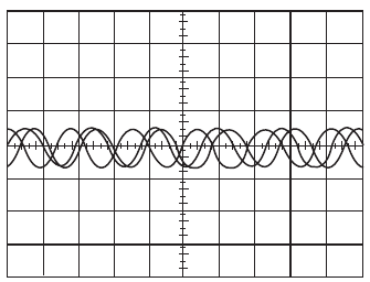
figure 13. Example of an un-triggered waveworm

Edge Triggering

The most basic and most common type of triggering is edge triggering. With edge triggering there are 2 main controls; the trigger ‘LEVEL’ knob and the trigger ‘Slope’ located in the ‘TRIG MENU’. The trigger circuit acts as a comparator. You select the slope and voltage level on one input of the comparator. When the trigger signal on the other comparator input matches your settings, the oscilloscope generates a trigger which initiates the sweep/capture of the waveform. The slope control determines whether the trigger point is on the rising or the falling edge of a signal. A rising edge is a positive slope and a falling edge is a negative slope. The level control determines where on the edge the trigger point occurs.

Trigger Level

The trigger level is the voltage that the input waveform must pass through to initiate a waveform capture. The trigger level is indicated in 2 different spots shown below. The first is located in the bottom right section of the display, it actually currently indicates 3 thing: The trigger input source ‘CH1’, the trigger edge ‘rising slope’ and the trigger voltage level ‘? V’.

figure 14. Trigger source, edge and voltage indicator

The second trigger level indicator is an arrow located on the right side of the display as shown below.

figure 15. Trigger position indicator

Trigger Menu

The trigger menu has the following options. The defaults are in bold and are typical settings.

• Type - (Edge/Video/Pulse)
  We will only be using the Edge type for our experiments.
• Source - (CH1/CH2/Ext/Ext/5/AC Line)
  This is what to use as the source for the trigger. Typically we will use either CH1, or possibly CH2.
• Slope - (Rising/Falling)
  This is the selection if you want to use a positive going edge or a going negetive edge to initiate your trigger. Typically we will use the ‘Rising’ edge unless specified otherwise.
  
• Mode - (Auto/Normal)
  We will always use Auto.
• Coupling - (DC/Noise Reject/HF Reject/LF Reject/AC)
  This is a coupling selection for the trigger. We will alway use DC.

4. Play with the trigger controls

   1. Adjust the trigger ‘LEVEL’ knob to see the results. Notice, if you move the trigger level above or below the peaks of the waveform what happens? The signal is no longer triggered.

   2. Enter the ‘TRIG MENU’ to see the different options.

      • Type - Notice that the other options don’t create a proper trigger for this waveform. But they do have their uses which we will not go into.
      • Source - As we only have channel 1 connected as an input this is the only source that we can currently use as a trigger source.
      • Slope - Select ‘Falling’ and see the result. The scope triggers on the other falling edge. Return to the ‘Rising’ Slope option.
      • Auto - Just leave this on Auto.
      • DC - Just leave this on DC.

3.1.2 The Function Generator

A function generator is a piece of electronic test equipment used to generate different types of repetitive voltage waveforms over a wide range of frequencies. Some of the most common waveforms produced by the function generator are the sine wave , square wave and triangular wave. Common function generators have controls to control the frequency, amplitude, DC offset, duty cycle and the waveform type. Below is an image of the function generators available in the laboratory.

figure 16. BK Precision 4011A Function Generator

Function Generator Controls

• Frequency - There are 3 separate controls for the frequency. You first need to select the approprite ‘Range’ as required using the range buttons. Then rotate the ‘Course’ knob until you get near the desired frequency and then use the ‘Fine’ control knob to zero-in on the desired frequency as close as possible.

• Waveform Type - Simply select the desired waveform type by pushing the appropriate button: Sine, Square or Triangular.

• Amplitude - Typically there is 2 Ranges for the amplitude. The normal range that goes up to approximately 10V and the -20dB range which is used when small voltages are required.

• Duty Cycle - Controls the duty cycle of the output waveform. There is usually a ‘calibrated’ position or button to allow for an exact 50% duty cycle.

• DC Offset - Allows you to add a DC offset to the output waveform. There is usually a ‘calibrated’ position or button to allow for an 0V DC offset.

5. Connect a BNC-to-banana plug lead to the function generator ‘OUTPUT’ and after removing the oscilloscope probe we have been using connect another BNC-to-banana plug lead to channel 1 of the oscilloscope. Connect the function generator output to channel 1 of the oscilloscope by connecting the 2 reds of the BNC-to-banana leads together, also connect the 2 blacks together. You need to change the Probe setting for Channel 1 on the oscillscope to 1X as that is what the BNC-to-banana plug leads are. Take some time to experiment with both the function generator and the oscilloscope so you become familiar with the controls. Try the different function generator button’s listed below and see if you can keep the waveform displayed properly on the screen without using ‘AUTOSET’. Displayed properly means at least 1 cycle up to about 10, The waveform should at least 3 division tall and not clipped off the screen as well as triggered properly.

   1. Try the different waveforms: Sine, Square and Triangular.

   2. Try to adjust the frequency using the different ranges and the course and fine knobs.

   3. Try to adjust the amplitude of the waveform. Note there is 2 different ranges.

   4. Try and add a DC offset to the waveforms. Note the ‘calibrated’ position.

   5. Try and adjust the duty cycle of the waveforms. Note the ‘calibrated’ position.

3.2 AC Resistor

7. Use the circuit below to demonstrate how a 100Ω resistor behaves while ac voltages of various frequencies are applied to it.

   

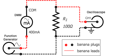
   figure 18. AC resistor test circuit

   1. Use a BNC-to-banana cable to connect the function generator as a variable frequency sinusoidal AC supply to the 100Ω resistor that is available on the student PCB, while also using a banana cable to also connect the digital multimeter as an AC milliammeter to measure the RMS current going through the resistor.

   2. Use another BNC-to-banana cable to connect channel 1 of the oscilloscope to measure the voltage across the resistor, make sure that the oscilloscope is set to use a 1X probe.

   3. While using the oscilloscope to view the voltage across the resistor adjust the function generator to output a 100Hz sinewave with no DC offset at maximum output voltage.

   Making Measurements on a Oscilloscope

   1. Method 1 - Counting Divisions
      Count the number of divisions a quantity spans across the screen of the oscilloscope and multiply it by the current value per division.
   2. Method 2 - Using Cursors
      Measure the change in quantity between the 2 cursors which need to be manually adjusted in either a horizontal (ie. time) direction or in a vertical (voltage) direction.
   3. Method 3 - Automatic Measurements
      The oscilloscope has the ability to make some measurements automatically by applying algorithms to the recorded waveforms. Caution is to be used while doing this as the oscilloscope can give you wrong values if it is not setup properly for that measurement type. Some of the time the oscilloscope will let you know if it isn’t confident in it’s value by having a question mark next to it’s quantity.

   4. Method 1 - Counting Divisions
      Follow these steps to measure the period and peak-to-peak magnitude of the sinewave using Method 1:

      1. Adjust the vertical ‘POSITION’ so the channel 1 ground indicator (the arrow on the far left side of the screen with the 1 next to it) is in the center of the screen.

      2. Adjust the horizontal ‘SEC/DIV’ so at least a complete single cycle of the sinewave is viewed on the screen and triggered properly.

      3. Adjust the ‘VOLTS/DIV’ so that the magnitude of sinewave is as large as possible without going off the screen.

      4. To measure the period of the sinewave, count the number of divisions on the screen of the oscilloscope that a single cycle of the sinewave spans and record that and the current seconds per division setting in the appropriate place on the results sheet. To obtain the period you simply need to multiply the number of divisions by the seconds per division, also record this in the appropriate place on the results sheet.

      5. To measure the peak-to-peak voltage of the sinewave, count the number of division on the screen that the magnitude of the sinewave spans (ie. from minimum to maximum) and multiply that by the current volts per division. Record all 3 of these values in the appropriate place on the results sheet.

   5. Method 2 - Using Cursors
      Follow these steps to measure the period and peak-to-peak magnitude of the sinewave using Method 2:

      1. Use the steps i-iii in Method 1 so your waveform is displayed properly.

      2. To use the cursors first push the ‘CURSOR’ button on the oscilloscope and then selecting ‘Type = Time’ and ‘Source = CH1’ by using the 5 buttons next to the CURSOR menu displayed on the screen. Notice that the 2 lights came on just below the vertical ‘POSITION’ knobs indicating to use those knobs to control the 2 cursors.

      3. To use the cursors to measure both the period and frequency of the sinewave use the now ‘CURSOR 1’ knob amd adjust it so it intersects the sinewave where the sinewave crosses through zero and then use the ‘CURSOR 2’ knob so that it intersects the sinewave also at the point where it crosses through zero but by 1 complete cycle (360°) away. Under the CURSOR menu on the display it shows ‘Delta’ which is the difference in time between the 2 cursors which is the period. It also shows 1/delta which in this case happens to be the frequency of the waveform. Record these values in the appropriate place on the results sheet.

      4. To use the cursors to measure the peak-to-peak amplitude of the sinewave change the ‘Type = Voltage’ and adjust ‘CURSOR 1’ so that it just touches the bottom of the sinewave. Adjust ‘CURSOR 2’ so that it just touches the top of the sinewave. The ‘Delta’ under CURSOR menu will now display the difference in voltage between the 2 cursors which is now the peak-to-peak amplitude. Record this value in the appropriate place on the results sheet.

   6. Method 3 - Automatic Measurements
      Follow these steps to measure the period, peak-to-peak and rms magnitude of the sinewave using Method 3:

      1. Use the steps i-iii in Method 1 so your waveform is displayed properly.

      2. You can also get the oscilloscope to make this measurement automatically by pushing the ‘MEASURE’ button and using the 5 buttons next to the screen to select one of the 5 measurements slots. For each slot you have the ability to make a different type of measurement for either channel. Using the appropriate button next to the display select: ‘Source = CH1’ and ‘type = Freq’ and the measured ‘Value’ should be shown underneath. Hit the ‘Back’ button to select another measurement if need be.

      3. On separate measurement slots select to measure ‘Freq’, ‘Period’, ‘Pk-Pk’ and ‘Cyc RMS’ for ‘CH1’ so the oscilloscope displays them all at the same time. Record these values in the appropriate place on the results sheet.

   7. Measure the rms current going through the resistor using the multimeter as an milliammeter and record this measurement in the appropriate place in the results sheet.

   8. Repeat the same measurements outlined in steps d-g with the function generator set to 1kHz and then again at 10kHz recording all results in the appropriate places on the results sheet.

3.3 AC Capacitors

8. Use the circuit below to demonstrate how a 68nF capacitor behaves while ac voltages of various frequencies are applied to it.

   

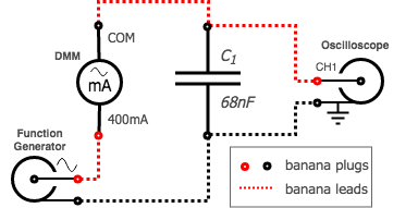
   figure 19. AC capacitor test circuit (68nF)

   1. Use a BNC-to-banana cable to connect the function generator as a variable frequency sinusoidal AC supply to the 68nF capacitor that is available on the student PCB, while also using a banana cable to also connect the digital multimeter as an AC milliammeter to measure the RMS current going through the resistor.

   2. Use another BNC-to-banana cable to connect channel 1 of the oscilloscope to measure the voltage across the capacitor.

   3. While using the oscilloscope to view the voltage across the capacitor adjust the function generator to output a 100Hz sinewave with no DC offset at maximum output voltage.

   4. Make sure the voltage sinewave waveform across the capacitor is displayed appropriately on the screen of the oscillscope and use the automatic measurements to measure both the frequency and RMS voltage applied to the capacitor. Record these results in the appropriate place in the results sheet.

   5. Measure the rms current going through the capacitor using the multimeter as an milliammeter and record this measurement in the appropriate place in the results sheet.

   6. Repeat the same measurements outlined in steps d-e with the function generator set to 1kHz and then again at 10kHz recording all results in the appropriate places on the results sheet.

9. Replace the 68nF capacitor with 1µF capacitor as shown in the circuit below.

   

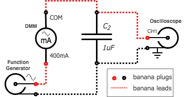
   figure 20. AC capacitor test circuit (1µF)

   1. Repeat the procedures in 8 for this new capacitor to obtain the results. Place your results in the appropriate place in the results sheet.

3.4 AC Inductor

10. Use the circuit below to demonstrate how a 2.5mH inductor behaves while ac voltages of various frequencies are applied to it.

    

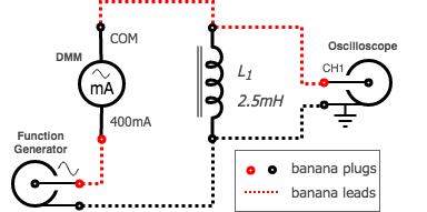
    figure 21. AC inductor test circuit (2.5mH)

    Note:
    The non-ideal resistance of this inductor is fairly high relative to it’s impedance at low frequencies and we will need to take this in to account while doing the calculations.

    1. Using a similar set of procedures as the capacitors above complete the appropriate section of the results sheet.

3.5 Series RC Circuit

11. Use the circuit below to demonstrate how the impedance of the series resistor-capacitor changes while ac voltages of various frequencies are applied to it.

    

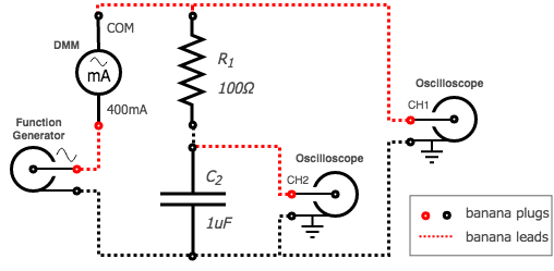
    figure 22. Series RC Circuit (Setup 1)

    1. Use a BNC-to-banana cable to connect the function generator as a variable frequency sinusoidal AC supply to the 100Ω resistor in series with the 1uf capacitor, while also using a banana cable to also connect the digital multimeter as an AC milliammeter to measure the RMS current coming from the function generator.

    2. Use another BNC-to-banana cable to connect channel 1 of the oscilloscope across the output of the function generator and milliammeter so the voltage across the combined impedance of the resistor and capacitor can be measured.

    Note:
    Channel 1 and Channel 2 both have a common ground. This means that you must connect the black lead of both channels to the same node of the circuit otherwise you will be creating a short circuit through the oscilloscope.

    3. Use yet another BNC-to-banana cable to connect channel 2 of the oscilloscope across the capacitor while making sure that both of the black leads coming from channel 1 and 2 of the oscilloscope are connected together. Turn on channel 2 of the oscilloscope by pushing the ‘CH 2 MENU’ button, you should notice a new arrow with a 2 beside it on the left side of the screen indicating the channel 2 ground (zero volt level). Make sure that you also configure the ‘Probe = 1X’ in the CH2 menu as that is what the BNC-to-banana plugs are.

    4. While using channel 1 of the oscilloscope to view the voltage output of the function generator adjust the function generators output to a 100Hz sinewave with no DC offset at maximum output voltage.

    5. Use the oscilloscope to measure and record the following in the appropriate place in the results sheet:

       • f_S: The frequency of the source voltage.

       • t_S: The period of the source voltage.

       • V_S^RMS: The rms voltage of the source.

       • V_C^RMS: The rms voltage across the capacitor.

       • t_C-S: The phase difference in time between the capacitor voltage and the source voltage.

       • V_C (Leads/Lags) V_S: Does the capacitor voltage lead or lag the source voltage.

    6. Measure the rms source current supplied to the circuit using the multimeter as an milliammeter and record this measurement in the appropriate place in the results sheet.

    7. Disconnect both oscilloscope probes from the circuit and reconnect them as shown below so we can now measure the voltage across the resistor and also have the source voltage as a reference for phase. In this case channel 1 is now measuring the source voltage but inverted from before. Channel 2 is now measuring the voltage across resistor but also inverted with respect to how we measured the capacitor. If you would like you can use the oscilloscope to invert both channels by going into the ‘CH 1 MENU’ and ‘CH 2 MENU’. You will notice that you end up with the same result either way. You need to do it this way because the 2 channels have a common ground.

    

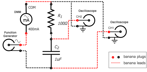
    figure 23. Series RC Circuit (Setup 2)

    8. Use the oscilloscope to measure and record the following in the appropriate place in the results sheet:

       • V_R^RMS: The rms voltage across the resistor.

       • t_R-S: The phase difference in time between the resistor voltage and the source voltage.

       • V_R (Leads/Lags) V_S: Does the resistor voltage lead or lag the source voltage.

    9. Repeat the same measurements outlined in steps e-h with the function generator set to 1kHz and then again at 10kHz recording all results in the appropriate places on the results sheet.

    10. For the last column on the results sheet you need adjust the frequency of function generator until the peak-to-peak voltage across the capacitor and resistor are the same. To do this you can use the ‘MATH MENU’ to display a 3rd waveform on the oscilloscope. As you are currently measuring the source voltage on channel 1 and the voltage across the resistor on channel 2 if you use the function ‘CH1-CH2’ that will show the voltage across the capacitor on the ‘MATH’ channel due to Kirchoffs Voltage Law. Using this ‘MATH’ feature adjust the oscilloscope settings and the function generator so the resistor and capacitor voltage have the same magnitude visually on the screen. Repeat the measurements again outlined in e-h with with these new settings and record your results in the appropriate place on the results sheet.

3.6 Series RL Circuit

12. Re-use the previous circuit replacing the 1µF capacitor with the 2.5mH inductor as shown below to demonstrate how the impedance of a series resistor-inductor changes while ac voltages of various frequencies are applied to it.

    

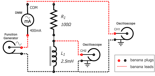
    figure 24. Series RL Circuit (Setup 1)

    1. Make all of the same measurements as the previous RC circuit and record the results in the appropriate place on the results sheet. Remember to move the oscilloscope probes in the same way you did for the previous circuit.

3.7 Clean-up

13. Cleanup your station, everything should be returned to where you got it from. Verify your results with an instructor or TA to show that you have completed everything and once everything is completed and tidy get a signature on your Results page before you leave.

4.1 Calculations

Complete the tables on your Results sheet by completing the following calculations:

1. For the AC Resistors section calculate the waveform period and the peak-to-peak voltage from your counting divisions measurements. Also calculate the resistance of the resistor by using your measured RMS voltage and RMS current.

2. For both AC Capacitors sections calculate both the reactance of the capacitor and the capacitance of the capacitor using your measured values.

3. For the AC Inductor section first calulate the inductors impedance using your measured values. Then, using the measured value of the non-ideal inductors resistance calculate the inductors reactance. Use this reactance to calculate the inductance of the inductor.

4. For the Series RC Circuit section calculate the following:

   1. The phase shift between the capacitor voltage waveform and the voltage source waveform.
   2. The phase shift between the resistor voltage waveform and the voltage source waveform.
   3. The sum of the 2 phase shifts in above to obtain the phase shift between the capacitor and resistor.
   4. The resistance of the resistor using ohm’s law for AC circuits and your measured values.
   5. The reactance of the capacitor using ohm’s law for AC circuits and your measured values.
   6. The total impedance of the resistor and capacitor is series by summing the 2 values calculated above.
   7. The total impedance again, this time using ohm’s law for AC circuits and your measured values.
   8. The capacitance of the capacitor using your measured values.
   9. The resistance of the resistor again, this time using the calculated impedance and the phase angle.
   10. The reactance of the capacitor again, this time using the calculated impedance and the phase angle.

5. For the Series RL Circuit section calculate all of the same things as the previous section with the following modifications.

   1. Only use ohm’s law for AC circuits to calculate R, Z_L and Z.
   2. Use the calculated Z_L and the measured resistance of the non-ideal inductor to find the inductors reactance (X_L).

4.2 Graphs

Using the provided graphs in your results sheet make the following plots:

1. Impedance-Frequency of R, L and C - Using your measurements and calculations from the AC Resistors, Capacitors and Inductors sections, plot each components resistance/reactance vs. frequency on the provided graph on your results sheet. Plot both the inductors reactance as well as it’s non-ideal impedance. Note that the plots x and y axes are both on logarithmic scales.

4.3 Questions

Answer the following questions on a separate piece of paper to hand in with your Results Sheet. Make sure to include an appropriate title, your first and last name, CCID, student ID and your lab section at the top of the page.

1. Explain how connecting the ground connections of each channel of an oscilloscope to different nodes in a test circuit can cause issues with your circuit. What are the potential dangers in doing this? Draw an example circuit to assist in your explanation.

2. Make some general observations and conclusions about how each of the different components on the plot Impedance-Frequency of R, L and C behave.

3. Looking at your results, does the inductor behave more like an ideal component at 100Hz or at 10kHz? Use what you know about a non-ideal inductor and your measurements as an example to explain your answer.

4. In your results for the Series RC circuit is the phase between the capacitor voltage and the resistor voltage approximately 90° as expected at all frequencies? Explain in your own words why this is expected?