Lab 5: Transient Analysis
ECE203 - Electrical Circuits II
Electrical and Computer Engineering - University of Alberta
1 Objectives
The objective of this lab is to study the transient response of several passive series circuits when a step voltage is applied to them. A transient response is the response of a system to a change from an equilibrium or a steady state. In this lab you will experiment with the following 3 circuits on a breadboard using the Analog Discovery 2 to create a step change in voltage and then to measure the result.
- A Series RC Circuit.
- A rising step change in voltage.
- A falling step change in voltage.
- Changing the capacitor value to see the effect on the rising step change in voltage.
- A Series RL Circuit.
- A rising step change in voltage.
- A Series RLC Circuit.
- A rising step change in voltage.
1.1 Equipment Required
- The Lab 5 - Results sheet to record your measurements.
- A Computer with Waveforms installed
- Analog Discovery 2
- Breadboard Breakout for the Analog Discovery 2 with a Ribbon Cable
- USB A to Micro-B cable
- Digital multimeter
- MB102 breadboard
- Jumper wires
- The following Resistors (1/4 watt, 1% or 5%)
- 100Ω resistor
- 1.0kΩ resistor
- 100nF capacitor
- 220nF capacitor
- 10mH inductor
1.2 Background
Resistors
As has been studied before, the application of a voltage \(V\) to a resistor (with resistance \(R\) in Ohms), results in a current \(I\), according to the formula: \[ I=\frac{V}{R} \] The current response to voltage change is instantaneous; a resistor has no transient response.
Inductors
A change in voltage across an inductor (with inductance \(L\) in Henrys) does not result in an instantaneous change in the current through it. The i-v relationship is described with the equation: \[ v=L\frac{di}{dt} \] This relationship implies that the voltage across an inductor approaches zero as the current in the circuit reaches a steady value. This means that in a DC circuit, an inductor will eventually act like a short circuit.
Capacitors
The transient response of a capacitor (with Capacitance \(C\) in Farads) is such that it resists instantaneous change in the voltage across it. Its \(i-v\) relationship is described by: \[ i=C\frac{dv}{dt} \] This implies that as the voltage across the capacitor reaches a steady value, the current through it approaches zero. In other words, a capacitor eventually acts like an open circuit in a DC circuit.
2 Procedures
2.1 Equipment Preparation
Use the Analog Discovery 2 and the Waveforms software to output a 400Hz Squarewave from the Wavegen tool and measure this output using the Scope tool.
- Use the provided USB A to micro-B cable to connect your Analog Discovery 2 to the USB port on your computer.

- Connect the one end of the ribbon cable with the notch in the proper orientation to the Analog Discovery 2 as shown below. Then connect the other end of the ribbon cable to the Breadboard Breakout using the supplied 15x2 header pins. Make sure that the orange wires of the ribbon cable end up on the same side as the breadboard breakout pin labeled 1+.

- Plug the breadboard breakout into the breadboard as a shown.

Connect the channel 1 Wavegen output to the channel 1 Scope input by connecting the following with jumper wires:
- Connect W1 to 1+
- Connect Gnd to 1-
.png)
Launch the Waveforms software making sure that it detects your Analog Discovery 2.
Step voltage source
The input voltage described in all the circuits during the lab have been described as a step voltage. This is most easily obtained by using the function generator set to deliver square waves. The rate of delivery of the step voltages is set to a time long enough that the circuit is allowed to reach a steady state before the voltage changes again. This effectively simulates a voltage source in series with a time-controlled on-off switch.
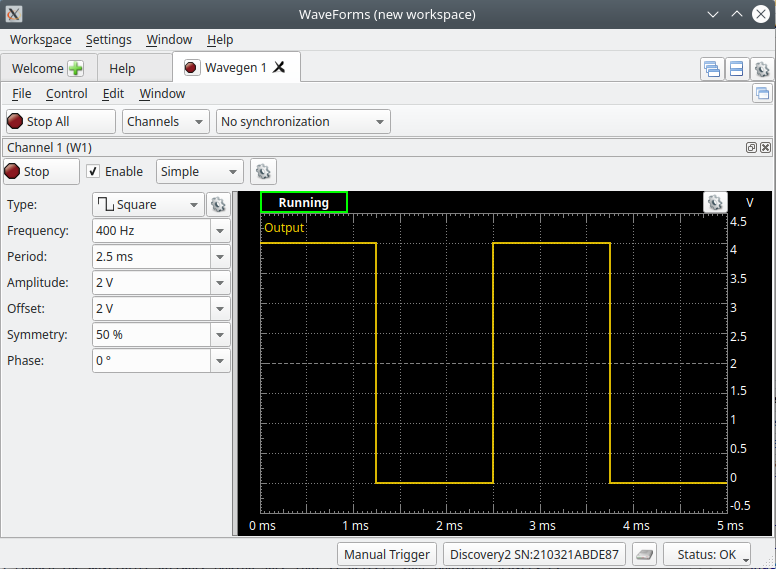
In Waveforms start the Wavegen tool and configure it with the following settings and once complete click on the ‘Run’ button to output the waveform on the W1 pin.
- Type: Square
- Frequency: 400 Hz
- Amplitude: 2 V
- Offset: 2 V
With the Wavegen tool still running launch the Scope tool with the following setting. Make sure to hit the ‘Run’ button to acquire the input waveform.
- Set the Trigger Level to 2V.
- Set the Base time to 500uS/div and the Position to 0s.
- Set the Channel 1 Offset to -2V and the Range to 500mV/div.
- Use the checkbox to turn off Channel 2.
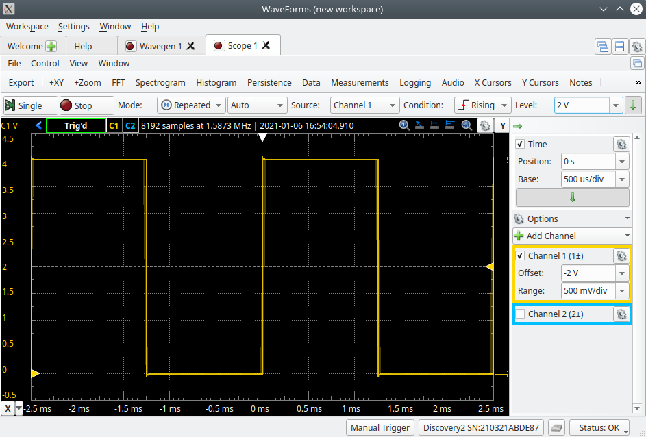
You should now notice that the waveform displayed on the Wavegen screen closely matches that which is being measured on the scope.
Temporarily ‘Stop’ both the Wavegen and Scope tools as you connect the circuit in the next part.
2.2 Series RC Circuit
Transient response of a series RC circuits
Solving the circuit below involves the solution of first and second order differential equations. Only the solution has been included, as that is all that is needed for the lab.
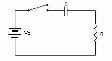
Figure 1.1: A Series RC Circuit
If the switch in this circuit was initially open, and then closed at time \(t=0\), the current in this circuit is: \[i(t)=I_O\ \exp\Big( \frac{-t}{\tau} \Big) \label{eq:eqa}\] where: \[I_O = \frac{V_O}{R} = \text{initial current after switch is closed}\ (\ t=0^+)\] \[\tau = RC = \text{is the time constant for the circuit}\] Another definition of \(\tau\) is obtained by setting \(t = \tau\) into \(\eqref{eq:eqa}\). Doing so gives \(i(\tau) = I_O\times(1/e)\). The time constant of an RC circuit is the time required for the current in the circuit to fall to \(1/e\) of its initial value.
Connect the circuit below using the following:
- Use the squarewave voltage source you configured in the last section as the source V1.
- Use the breadboard to connect a 100nF capacitor (C1) in series with a 1.0kΩ resistor (R1) to the voltage source (V1).
- Use the the Scope’s channel 1 (1+, 1-) and channel 2 (2+, 2-) inputs to measure Vin and Vout respectively.

Figure 1. Series RC Circuit
Click here
to see a simulation
demo of this circuit.
Once connected your breadboard should look something like the following.
.png)
With the circuit now connected click on the ‘Run’ button in both the Wavegen and Scope tools. You should now be able to see the Vin waveform displayed on the Scope screen as before. Make the following changes to in the Scope tool.
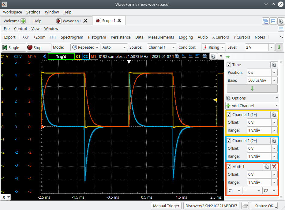
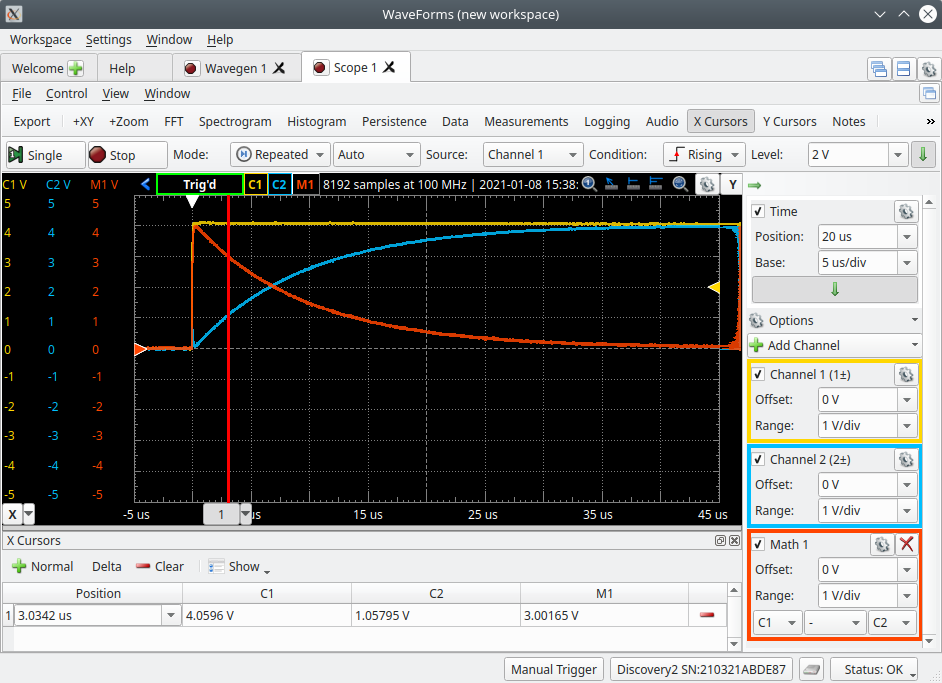
Adjust Channel 1 so the Offset is 0V and the Range is 1V/div. Channel 1 is displaying the waveform of the source voltage (V1) in yellow.
Turn on Channel 2 using the appropriate check box and set its Offset to 0V and its Range to 1V/div. Channel 2 is displaying the voltage across the resistor (R1) in blue.
As the voltage across the capacitor (C1) is simply the source voltage (V1) minus the voltage across the resistor (R1) due to kirchoffs voltage law, we can use the math capabilities of the Scope tool to also display this waveform. To do this select the ‘Add Channel’ dropdown menu and select ‘Simple’ and a new channel labelled ‘Math 1’ will be created. For the ‘Math 1’ channel we want to have it take channel 1 (the source voltage) and subtract channel 2 (the resistor voltage). This can be selected using the dropdown menus in the ‘Math 1’ control box, where ‘C1’ and ‘C2’ are short for channel 1 and channel 2 respectively, and the center downdown is the sign where you can select ‘-’.
Adjust the ‘Math 1’ channel Offset to 0V and the Range to 1V/div to match the other channels. The ‘Math 1’ channel is now displaying the voltage across the capacitor (C1) in red.
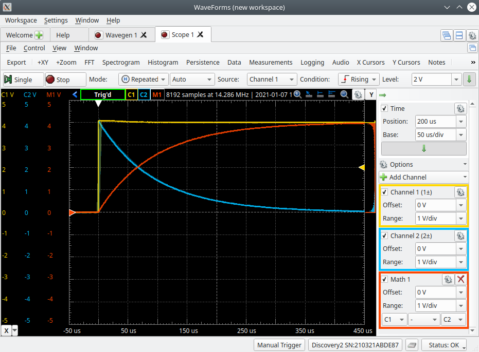
Your Scope should now look like the following image. Take a minute and try and understand what is going on with these waveforms. Note that this is a series circuit that the current waveform will look identical to the resistor voltage (the blue waveform) only 1000 times smaller in magnitude due to the resistor being 1kΩ. Another thing to note is that both the source voltage (yellow) and the capacitor voltage (red) are always positive, where the resistor voltage and circuit current is either positive or negative depending on weather the source voltage just turned on or off.
Now that we want to measure how the capacitor voltage rises with time when the source voltage is stepped from 0V to 4V, we want to make this rise as large as possible on the display to obtain accurate measurements.
Change the Scopes Time Base from 500us/div to 50us/div. This makes the rise less sharp but it now goes off the edge of the screen before it finishes charging.
To compensate for the capacitor voltage going off the edge of the screen before it finishes charging we are also going to move the trigger position to the left. First note the white triangle indicator pointing down at the top of the display. This indicator is where the waveform is triggered and also denotes the time zero seconds. Also note the time marking at the bottom of the display. To move the indicator you can either click on it and drag it horizontally to either the left or right or use the Position dropdown in the Time controls. Lets select a 200us position which will move the indicator and waveforms 4 divisions to the left.
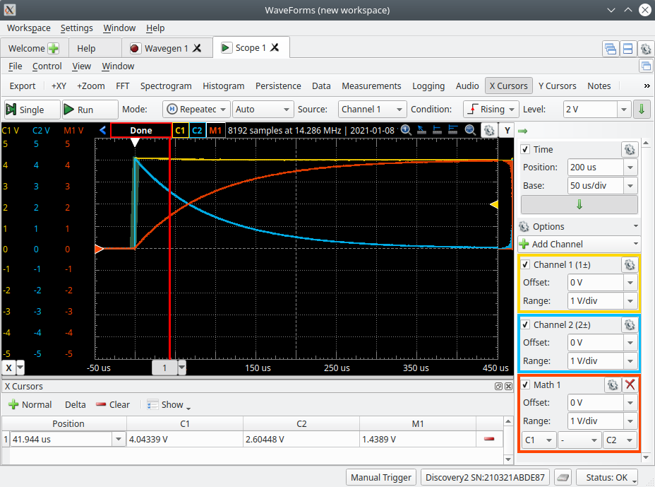
Your Scope should now look like the following image.
Apply a rising step change in source voltage to a series RC circuit. Measure the capacitors voltage at multiple times as it charges. We will also measure the resistor and supply voltage for completeness. To make these measurements we are going to use the “X Cursors’ tool.
- Open the ‘X Cursor’ tool by selecting it on the toolbar and it should open up a new tool as shown below somewhere on the page.
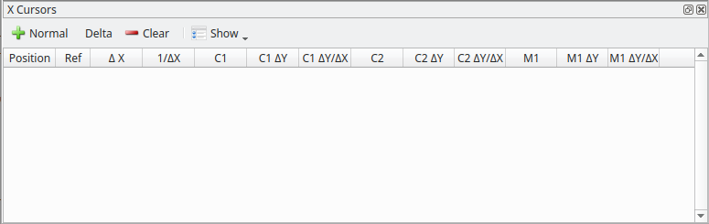
- Add a cursor by selecting the ‘Normal’ button and a new red cursor will be be displayed on the oscilloscope and a new line will be added in the ‘X Cursors’ display. As we are only interested in the voltage of the 3 waveforms at the cursors position and the time at the cursor, we can hide all of the other cells in the X Cursors display by clicking on the ‘Show’ dropdown and deselecting everything but Position, C1, C2 and M1. As the Scope is continuously acquiring new data the measured values in the X Cursor window are constantly changing. If you would like to read the values from a static number you can either click on the ‘Single’ or ‘Stop’ button at the top left of the Scope.
Using the cursors record the voltage across the source (V1), capacitor (C1) and resistor (R1) at the following times relative to the rising step change in source voltage and record the measurements on your results sheet:
- -1us (just before the step)
- 1us (just after the step)
- 10us
- 20us
- 50us
- 100us
- 200us
- 500us (Adjust the Time Base and/or Position so this time is displayed on the Scope)
- 1000us (Adjust the Time Base and/or Position again so this time is displayed on the Scope)
Measure the time constant (τ) of this RC circuit.
To measure the time constant we need to measure the time it takes for the current to fall to (1/e) of its initial (peak) value right after the step change in source voltage. Remember that the current waveform will look identical to the resistor voltage. We can assume that the initial resistor voltage will be equal to the source voltage just after the step and as the capacitor charges the resistor voltage (and current) will fall.
For example:
If the source voltage is 4V how long does it take the resistor voltage to fall to 1/e (~0.3679) of its initial value, or to 1.472V.
Measure the time constant (τ) using the X Cursors and record your measurement in the appropriate place on the results sheet.
Calculate the theoretical time constant (τ) of this circuit and place your result in the appropriate place in the results sheet.
To compare a rising step change to a falling step change make the same measurements as before but now with a falling step change in source voltage which will cause the capacitor to discharge.
- With the Scope running again change the trigger ‘Condition’ to ‘Falling’ which will cause the scope to trigger on the source voltages falling edge which will now be the reference time of zero seconds. You may need to adjust your scope setting to obtain the required measurements.
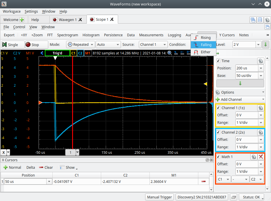
- Using the cursors again measure the voltage across the source (V1), capacitor (C1) and resistor (R1) at the same times as before making sure to record your measurements in the appropriate place on the results sheet.
Compare how a larger capacitance in an RC circuit effects the rate at which the voltage increases across the capacitor when a rising step voltage is applied.
Replace the 100nF capacitor (C1) with a 220nF capacitor.
With the trigger ‘Condition’ set to ‘Rising’ use the cursors to measure the same voltages at the same times in a similar manner as you did for the 100nF capacitor. Record your measurements in the appropriate place in the results sheet.
Measure the new time constant of this new circuit. Record your measurement in the appropriate place in the results sheet.
Temporarily ‘Stop’ both the Wavegen and Scope tools as you connect the circuit in the next part.
2.3 Series RL Circuit
Transient response of a series RL circuits
Solving the circuit below involves the solution of first and second order differential equations. Only the solution has been included, as that is all that is needed for the lab.
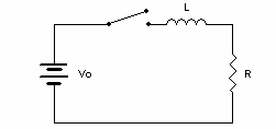
Figure 1.2: A Series RL Circuit
If the switch in this circuit is initially open, and then closed at time \(t=0\), the current in this circuit will be described as: \[i(t)=I_O(1-e^{-t/\tau}) \label{eq:eqb}\] where: \[I_O=\frac{V_O}{R}= \text{the limiting value of the current in the circuit}\] \[\tau=\frac{L}{R}=\text{is the time constant for the circuit}\] \(\tau\) can also be described by noting what happens when \(t = \tau\) is substituted into \(\eqref{eq:eqb}\). Doing so gives \(i(\tau) = I_O\times(1-1/e)\). In other words, \(\tau\) is the time required in an RL circuit for the current to grow to \((1-1/e)\) of its limiting value.
Modify the circuit from before to obtain the following:
- Use the same squarewave voltage source you configured in the last section as the source V1.
- Use the breadboard to connect a 10mH inductor (L1) in series with a 1.0kΩ resistor (R1) to the voltage source (V1).
- Use the the Scope’s channel 1 (1+, 1-) and channel 2 (2+, 2-) inputs to measure Vin and Vout respectively.

Figure 2. Series RL Circuit
Click here
to see a simulation
demo of this circuit.
With the Wavegen and Scope tools running make sure that the Scope is configured correctly to display all 3 of the required waveforms: The source voltage (yellow), the resistor voltage (blue) and the inductor voltage (red). Adjust the Time Position and Base and any other Scope controls so the inductor voltage transient takes up most of the screen. Just like the last circuit note that this is also a series circuit and the current waveform will look identical to the resistor voltage (the blue waveform) only 1000 times smaller in magnitude due to the resistor being 1kΩ. Once complete is should look something like below.
Using the cursors record the voltage across the source (V1), resistor (R1) and inductor (L1) at the following times relative to the rising step change in source voltage and record the measurements on your results sheet:
- -200ns (just before the step)
- 200ns (just after the step)
- 2us
- 5us
- 10us
- 20us
- 50us
- 100us (Adjust the Time Base and/or Position so this time is displayed on the Scope)
Measure the time constant (τ) of this RL circuit.
To measure the time constant we need to measure the time it takes for the current to grow to (1-1/e) of its limiting value which will be the source voltage divided by all of the resistance in the circuit. Remember that the current waveform will look identical to the resistor voltage. We can assume that the initial resistor voltage (and current) will be equal to the zero and as the inductor charges the resistor voltage (and current) will increase.
For example:
If the source voltage is 4V how long does it take the resistor voltage to increase to 1-1/e (~0.6321) from its initial value, or to 2.528V.
Measure the time constant (τ) using the X Cursors and record your measurement in the appropriate place on the results sheet.
Calculate the theoretical time constant (τ) of this circuit and place your result in the appropriate place in the results sheet.
Temporarily ‘Stop’ both the Wavegen and Scope tools as you connect the circuit in the next part.
2.4 Series RLC Circuit
Transient response of a series RLC circuit
Solving the circuit below involves the solution of first and second order differential equations. Only the solution has been included, as that is all that is needed for the lab.
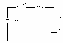
Figure 1.3: A Series RLC Circuit
In theory, there are three cases for the way a series RLC circuit will respond when the switch is closed at time \(t=0\). In this lab, only the underdamped case will be dealt with. For this case, the current in the circuit is described by: \[i=\frac{V_O}{\omega_d L}\ \exp(-\alpha t)\ \sin(\omega_d t) \label{eq:eqc}\] where \[\omega_d=\sqrt{\omega_0^2-\alpha^2}\] \[\omega_0=\frac{1}{\sqrt{LC}}\quad \text{and} \quad \alpha=\frac{R}{2L}\] Equation \(\eqref{eq:eqc}\) describes a current that is both fluctuating and deteriorating, as shown in Figure 1.4:
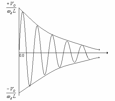
Figure 1.4: The Current in an Underdamped Series RLC Circuit
The current in the circuit oscillates due to the sine component in Equation \(\eqref{eq:eqc}\), but the maximum value it can reach is decaying due to the negative exponential. The “envelope” that the current must fall within is described by: \[i=\pm \frac{V_O}{\omega_d L}\ \exp(-\alpha t) \quad \text{or} \quad |i|=\frac{V_O}{\omega_d L}\ \exp(-\alpha t)\] The quantity \(\alpha\) is referred to as the time constant of the envelope. It is determined by taking the natural logarithm of both sides of the above equation: \[\ln|i|=\ln \frac{V_O}{\omega_d L}-\alpha t\] which is a linear equation. If a graph of \(\ln|i|\ \text{vs.}\ t\) is plotted, its slope will be \(–\alpha\).
Resonance of an RLC circuit
The resonant frequency of an RLC Circuit is the frequency at which current is a maximum. This occurs when the impedance of the capacitor equals the impedance of the inductor. \[|\overline{Z_C}|=|\overline{Z_L}|\] \[\bigg|\frac{1}{j\omega_OC}\bigg|=|j\omega_OL|\] At this frequency, the impedance of the capacitor (negative) exactly cancels the impedance of the inductor (positive). The only impedance felt by the source is the resistor. It follows that the current at this frequency will be in phase with the voltage source, and at a maximum magnitude.
Modify the circuit from before to obtain the following:
- Use the same squarewave voltage source you configured in the last section as the source V1.
- Use the breadboard to connect a 100nF capacitor (C1), 10mH inductor (L1) and a 100Ω resistor (R1) in series to the voltage source (V1).
- Use the the Scope’s channel 1 (1+, 1-) and channel 2 (2+, 2-) inputs to measure Vin and Vout respectively.

Figure 3. Series RLC Circuit
Click here
to see a simulation
demo of this circuit.
With the Wavegen and Scope tools running make sure that the Scope is configured correctly to display all 3 of the required waveforms: The source voltage (yellow), the resistor voltage (blue) and the inductor+capacitor voltage (red). We won’t be measuring the inductor and capacitor voltage separately but if you would like to see what they look like I would suggest looking at the demo simulation. Adjust the Time Position and Base and any other Scope controls so you can view 2 squarewave cycles on the Scopes display. Just like the last circuit note that this is also a series circuit and the current waveform will look identical to the resistor voltage (the blue waveform) this time only 100 times smaller in magnitude due to the resistor being 100Ω. Once complete is should look something like below.
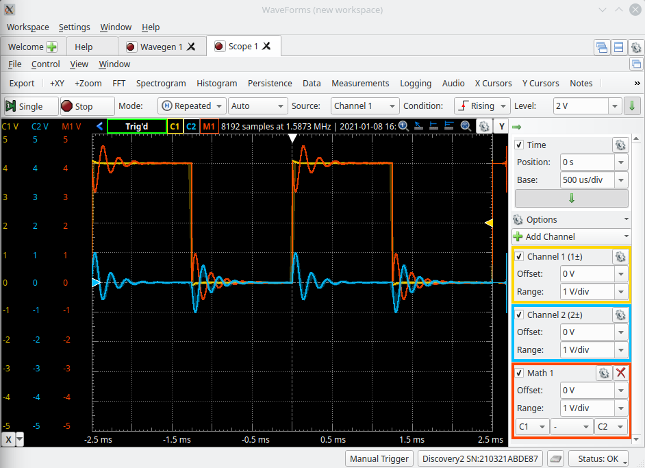
As we want to examine the oscillating current after the rising step in the source voltage we are going to look at the resistor voltage.
Turn off the Channel 1 and the Math 1 Channel by using the check box controls.
Use the Time and Channel 2 controls to make one ringing event take up as much as of the Scopes display as possible. You will need at least 3 complete ringing cycles displayed on the screen. It should now look something like below.
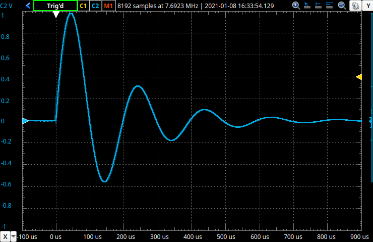
Use the ‘X Cursors’ to measure the following for the first 3 cycles of the ringing/oscillating event. Record your measurements in the appropriate place in the results sheet.
- The time when the cycle crosses 0V while rising or starts oscillating for the initial cycle. (ie. rising zero)
- The time and magnitude of the positive peak voltage. (ie. positive peak)
- The time when cycle crosses 0V while falling. (ie. falling zero)
- The time and magnitude of the negative peak voltage. (ie. negative peak)
2.5 Cleanup
Congratulations, you have completed the experimental part of the the laboratory. Before cleaning up, I’d suggest going through your results to check that you have completed everything and that your results make sense. If you find any issues, I’d suggest resolving or making a note of it now. If you are not continuing to work with the equipment please disconnect everything and put it away to prevent it from getting damaged.
3 Post Lab
The following is what you are expected to complete and submit for grading for Lab 5 before the deadline .
The completed Lab 5 - Results sheet template provided at the beginning of this lab manual under Equipment required. This sheet should include the following:
- Your name, student ID and CCID.
- All of the required measurements from the lab procedures.
- All of the required calculations as discussed below.
- The required plots as discussed below.
The Lab 5 - Results sheet needs to be submitted to the Submit (Lab 5 - Results) link on eClass as a pdf document .
- Complete the online Quiz (Lab 5 - Post Lab) on eClass.
3.1 Calculations
For these calculation you only need to provide the answers in the space provided on your results sheet, you do not need to show your work.
Calculate the theoretical time constant (τ) for two Series RC Circuits and the Series RL Circuit. Record your answers in the appropriate place in the results sheet to compare with your measurement.
Calculate the frequency of ringing for each cycle for the first 3 cycles you measured for the Series RLC Circuit. Use one zero crossing to the next to determine the period of the cycle and use that period to calculate the frequency. Record your answers in the appropriate place in the results sheet.
Calculate the theoretical Resonant frequency for the Series RLC circuit and record your answer in the appropriate place in the results sheet to compare with the measured ringing frequency.
3.2 Plots
To create your plots you can use whichever software you would like (Excel, Matlab, etc), export your plot as an image and import it into your Lab 5 - Results sheet in the appropriate place.
Your plots should include:
- A Plot title
- Label your axes and show what unit of measure is used.
- Include a marking for your datapoints.
- Include a line between your datapoints in the same series.
- Include a legend.
- Make sure your scales are appropriate and visible.
Note:
When looking at your plots remember that the current waveform looks identical to the resistor voltage waveform which is just scaled by the resistor value.
Series RC Circuit (1kΩ and 100nF/220nF) - Rising Edge: Plot the source voltage, resistor voltage and capacitor voltage vs. time. Add the 220nF capacitor voltage vs. time to the plot to compare this waveform to the 100nF capacitor voltage waveform.
Series RC Circuit (1kΩ and 100nF) - Falling Edge: Plot the source voltage, resistor voltage and capacitor voltage vs. time.
Series RL Circuit (1kΩ and 10mH) - Rising Edge: Plot the source voltage, resistor voltage and inductor voltage vs. time.
Series RLC Circuit (Ringing) - Absolute Peaks: Plot the absolute value of the voltage peaks you measured across the resistor vs. time.
3.3 Questions
Complete the online Quiz (Lab 5 - Post Lab) on eClass.