Lab Tutorial: Equipment
ECE203 - Electrical Circuits II
Electrical and Computer Engineering - University of Alberta
1 Objectives
This tutorial will show you how to get started with the Analog Discovery 2 which will be used extensively throughout this course. It will start off by getting it connected to your computer and installing the required software. It will then continue by introducing you to the main tools on the device that will be used throughout this course: The DC Power Supply, the Voltmeter, the Waveform Generator and the Oscilloscope.
1.1 Equipment Required
- Analog Discovery 2
- Breadboard Breakout for the Analog Discovery 2 with a Ribbon Cable
- A USB A to Micro-B cable
- MB102 breadboard
- Jumper Wires
1.2 Background
2 Analog Discovery 2
The Digilent Analog Discovery 2™, developed in conjunction with Analog Devices®, is a multi-function instrument that allows users to measure, visualize, generate, record, and control mixed signal analogue and digital circuits. The low-cost Analog Discovery 2 is small enough to fit in your pocket, but powerful enough to replace a stack of lab equipment, providing engineering students, hobbyists, and electronics enthusiasts the freedom to work with analogue and digital circuits in virtually any environment, in or out of the lab.
2.2 Connections
Connect the Analog Discovery 2.
- Use the provided USB A to micro-B cable to connect your Analog Discovery 2 to the USB port on your computer.

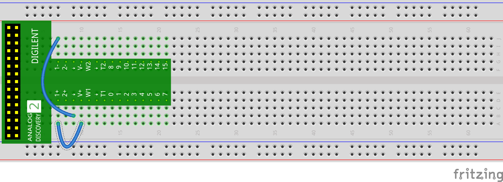
- Connect the one end of the ribbon cable with the notch in the proper orientation to the Analog Discovery 2 as shown below. Then connect the other end of the ribbon cable to the Breadboard Breakout using the supplied 15x2 header pins. Make sure that the orange wires of the ribbon cable end up on the same side as the breadboard breakout pin labeled 1+.

- Plug the breadboard breakout into the breadboard as a shown.

2.3 DC Power Supply
Use the DC Power Supply on the Analog Discovery 2.
Watch the short video on how to use the DC Power Supply on the Analog Discovery 2.
Start the ‘Waveforms’ software for the first time.
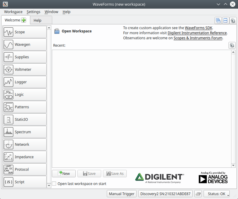
If everything is connected and installed correctly you should notice the device and serial number (SN:) in the bottom corner as well as the devices status (OK).
The first tab displayed should be the welcome screen. All of the available tools on the device are located along the left side of this tab. Click on the “Supplies” button and a new tab will open with the controls for the Supplies.
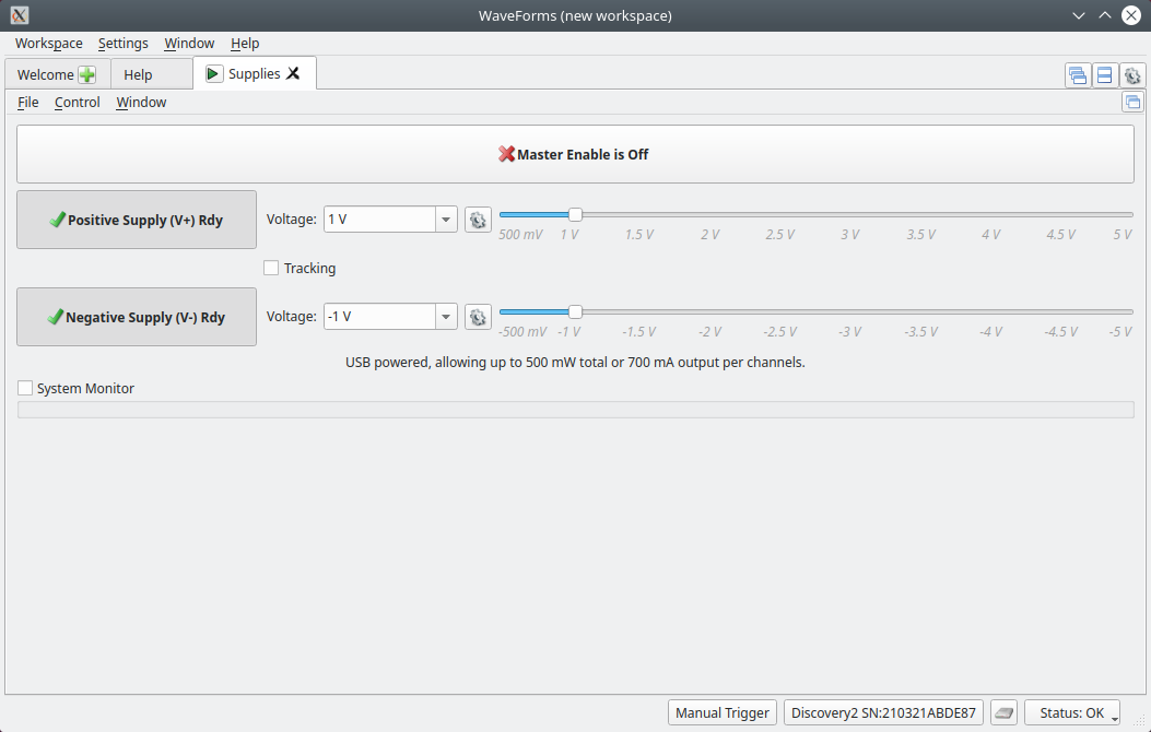
The Analog Discovery 2 is equipped with two DC power supplies: 1 positive supply and 1 negative supply.
Both power supplies should currently be disabled as the “Master Enable is Off”.
By clicking on the “Master Enable” both supplies will then output the corresponding voltage for that supply on it’s designated output pins: (V+ and Gnd/) and (V- and Gnd/) for the positive and negative supplies respectively.
Note:
On the Analog Discovery 2 they show the circuit ground or circuit common of the device with a ground symbol or down arrow (), it can also be abbreviated as Gnd. There are 4 of these on the Analog Discovery 2 and they are all a common ground node.Each supply has its own enable as well.
To control the output voltage of the supply you can either use the drop down to select a voltage, type the number to 3 decimal places or use the slider. The positive V+ has a range from 500mv to 5.0V while the Negative V- is from -500mv to -5.0V
There is also a “Tracking” checkbox, when this is enabled the positive and negative voltage will always have the same absolute value. In this mode you can use any of the controls to set both output voltages.
Go ahead and play with the Supplies controls to test them out to see how they function.
2.4 Voltmeter
Use the Voltmeter on the Analog Discovery 2 to measure the output of the voltage supply on the Analog Discovery 2.
Watch the short video on how to use the Voltmeter on the Analog Discovery 2.
Use 2 jumper wires to make the following connections on the breadboard.
- V+ to 1+
- Gnd/ to 1-
- From the Welcome screen start the “Voltmeter” tool to open the controls for the Voltmeter.
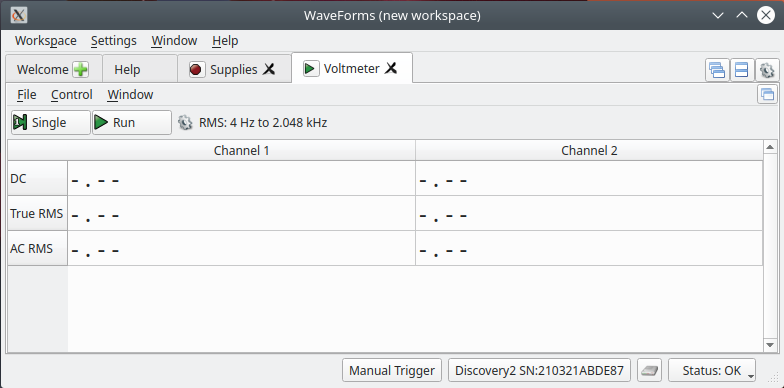
The Analog Discovery 2 is equipped with 2 voltmeters: Channel 1 and Channel 2.
Both voltmeters should currently be disabled as they are not running.
By clicking on the “Run” button both voltmeters will then display the corresponding voltage that is currently measuring on its input pins: (1+ and 1-) and (2+ and 2-) for Channel 1 and Channel 2 respectively. The measurements are updated at a certain refresh rate continuously.
Hitting the same button again, now “Stop”, will stop the acquisitions.
There is also a “Single” acquisition button that will acquire a single measurement and then stop on its own.
With each acquisition there are 3 values that are calculated: DC, True RMS, AC RMS. The reading we will use for this lab is the DC reading. You will learn what the difference of these readings are later in this course.
Using both the “Supplies” and “Voltmeter” controls see if you can generate a voltage using the positive supply and measure it using channel 1 of the voltmeter. Try changing the voltage and measuring again. Play with all of the “Supplies” and “Voltmeter” controls until you are familiar with them.
Note
You can enable or disable a tool from the tab by clicking on the green triangle to enable and the red square to disable.
2.5 Wavegen
Learn to use the Wavegen tool of the the Analog Discovery 2.
Watch the short video on how to use the Waveform Generator on the Analog Discovery 2.
Connect the Analog Discovery 2 to the computer and to your breadboard like you have done in the previous labs.
Open the ‘Waveforms’ program and make sure that it successfully connected to your Analog Discovery 2.
Select the Wavegen tool from the left-side menu and you should get a new tab that looks like the following.
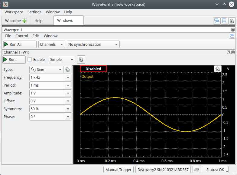
Wavegen
The main window shows a single cycle of the waveform that will be output to the Wavegen channel 1 output pins (W1 and Gnd) when the tool is running.
You can adjust the output waveform by either typing a value or using the dropboxes on the left-side controls menu. The ‘Simple’ controls are as follows:
- Type: The type of waveform (Sine, Square, Triangle etc…)
- Frequency: The frequency of the waveform. (= 1/Period)(10MHz maximum)
- Period: The period of the waveform. (= 1/Frequency)
- Amplitude: The peak AC component amplitude of the waveform.
- Offset: The DC component that is added to the AC waveform.
- Symmetry: How symmetrical the positive and negative sides of the AC waveform are. (50% is normal)
- Phase: At what phase the waveform starts.
To output the currently displayed waveform on the corresponding output pins you need to hit the ‘Run’ Button in the upper left-hand corner. Once it is running the ‘Run’ button becomes the ‘Stop’ button.
Without hitting the ‘Run’ button you can preview what the output waveform will look like. You can go ahead and use the controls to see how each one effects the display of the waveform.
2.6 Scope
The oscilloscope or “scope” is one of the most versatile and heavily used electronic measuring instruments in science, engineering, and industry. The oscilloscope earns its status as an important instrument because it neatly graphs how voltage varies as a function of time. Time varying voltage signals are not only important in electronic devices but also useful in measuring all kinds of other types of signals that are converted into an electrical signal by a transducer. A transducer is a device that converts one type of energy to another.
Watch the short video on how to use the Oscilloscope on the Analog Discovery 2.
Learn to use the Scope tool of the Analog Discovery 2 by using the Wavegen tool as a AC voltage source that can be measured and displayed with channel 1 of the Scope tool.
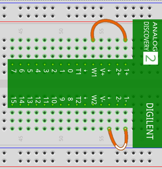
scope connections
Connect the Wavegen 1 output to the channel 1 input of the scope as shown in the circuit above by connecting the following:
Connect the Wavegen output (W1) to the positive channel 1 input (1+) of the Scope.
Connect the Wavegen output (Gnd) to the negative channel 1 input (1-) of the Scope.
From the Welcome tab in Waveforms select the Scope tool from the left-side menu and you should get a new tab that looks like the following.
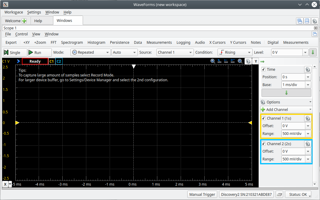
Scope
Run the Wavegen tool to output a 1kHz sinewave at 1V amplitude and then also Run the Scope tool with its default settings. You should now have something like the following.
Note:
In Waveforms to view both the Wavegen tool and the Scope tool at the same time as shown above you can click on the middle button in the upper right hand corner of the screen when both tools are already open.

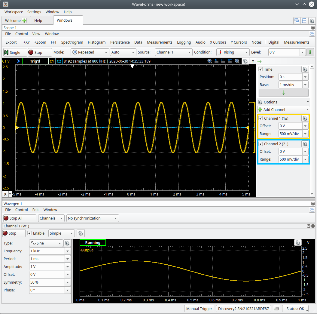
Scope/Wavegen split
A typical Oscilloscope has 3 main control sections: Vertical, Horizontal and Trigger. These controls section will be discussed in the following sections.
2.6.1 Vertical Section
The vertical section controls the y-axis of the displayed incoming voltage signal. There is one set of controls for every input channel. In our case since this is a 2-channel oscilloscope there are 2 sets of controls. The main vertical controls are ‘Offset’ and ‘Range’ which contribute to how the incoming waveform is displayed on the vertical/y-axis.
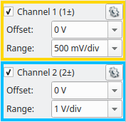
Vertical section controls
The key points about the vertical/y-axis are:
- There are 2 vertical channels: channel 1 in yellow and channel 2 in blue.
- The channels can be turned on and off using the checkbox next to the Channel name.
- It is the voltage axis. The higher the incoming voltage, the farther from the ‘ground’ (0 Volt level) the graph moves for a given ‘Range’ setting.
- Voltage can be positive or negative relative to ‘ground’. Positive input voltages moves the graph point above the ‘ground’; negative input voltage moves it below the ‘ground’.
Vertical Position
Each input channel has a ‘ground’ (0 Volt level) indicator on the left edge of the screen. Below is an image showing the vertical position of channel 1 which should now be in the vertical center of the display.

Vertical position indicator
The ‘Offset’ dropdown box or clicking and dragging the indicator will move this position indicator up and down on the display which in turn will also move the incoming voltage waveform up and down on the display.
Note:
All of the controls on the Scope have no effect on the incoming voltage it only effects the way the waveform is displayed on the screen.
Volts per Division
A typical oscilloscope will have 8-10 vertical divisions on the display. You can change the graph’s y-axis scale (usually expressed in volts per division or VOLTS/DIV) using the Range dropdown box to control how the incoming voltage waveform is scaled when it is displayed on the graph.
The displayed waveform (currently 2V peak to peak) should currently span approximately 4 vertical divisions of the oscilloscope’s screen if the range is currently set to 500mV/div. When you multiply the number of vertical divisions the waveform spans (~4) by the VOLTS/DIV setting (500mV/div) you arrive at that peak to peak voltage (2Vp-p).
Adjust Vertical
Adjust the following Channel 1 vertical controls to see how they effect the Scopes graph display.
Make a change to the ‘Offset’ dropdown box to other values and see the result. It should move the waveform and the ‘ground’ indicator up and down on the screen. You can also try clicking and dragging on the indicator to see the results. Return the position back to the center of the display by setting the offset to 0V.
Make a change to ‘Range’ dropdown box and see result. It should scale the magnitude of the waveform on the screen. Return the ‘Range’ back to 500mV/div.
2.6.2 Horizontal Section
The horizontal section controls the x-axis, which is generally used as the time-axis. There is only one common set of controls for all of the input channel. The horizontal controls are ‘Position’ and ‘Base’ which all contribute to how the incoming waveform is displayed on the horizontal/x-axis.
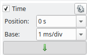
Horizontal section controls
The key points about the x-axis are:
- The x-axis is generally a time axis. In that mode, the point on the screen sweeps across at a constant user selectable speed, covering equal distances across the screen in equal times.
- If there is no input signal, you will see a horizontal line at y = 0, usually in the center of the display.
- Changing the ‘Base’ or ‘Sec/div’ changes the scale of the x-axis on the graph display.
- Time is scaled in units of seconds/division (Sec/div). To rescale the time axis, use the ‘Base’ control dropbox.
Horizontal Position
The current horizontal position is indicated on the top edge of the graph, typically in the center of the display which represents 0 seconds. This mark indicates where the current captured waveform was triggered. Below is an image showing the horizontal position of the display.

Horizontal position indicator
The ‘Position’ dropdown box or clicking and dragging the indicator will move this position indicator left and right on the display which in turn will also move the incoming voltage waveform left and right on the display.
Seconds per Division
A typical oscilloscope will have 10 horizontal divisions on the display. You can change the graph’s x-axis scale (expressed in seconds per division or Sec/div) using the ‘Base’ dropdown box to control how the time-base of the incoming voltage waveform is scaled when it is displayed on the graph.
Adjust Horizontal
Adjust the horizontal controls to see how they effect the Scopes graph display.
Make a change to the ‘Position’ dropdown box to other values to see the result. It should move the waveform and the position indicator left and right on the screen. You can also try clicking and grabbing the indicator to see the result. Return the position back to the center of the display by setting the ‘Position’ back to 0s.
Make a change to the ‘Base’ dropdown box to see result. It should scale the time base of how the waveform is displayed on the screen. Return the ‘Base’ back to 1ms/div.
2.6.3 Trigger Section
An oscilloscope’s trigger function synchronizes the horizontal sweep at the correct point of the signal, essential for clear signal characterization. Trigger controls allow you to stabilize repetitive waveforms and capture single-shot waveforms. The trigger makes repetitive waveforms appear static on the oscilloscope display by repeatedly displaying the same portion of the input signal. Imagine the jumble on the screen that would result if each sweep started at a different place on the signal, as illustrated the figure below.

Example of an un-triggered sinewave
Trigger Controls

Trigger section controls
Along the Trigger controls toolbar you have the following controls:
Single - When the ‘Single’ button is pushed the acquisition will wait for a trigger signal to occur and then capture a single acquisition from the inputs, automatically stopping after the acquisition is complete.
Run/Stop - When the ‘Run’ button is pushed the acquisition will wait for a trigger signal to occur and then capture an acquisition from the inputs. Once the first acquisition is finished it will then wait for another trigger signal to start the next one. This will happen indefinitely until the ‘Stop’ button is pushed.
Mode: - These are more advanced settings that will not be used in this course. For our purposes they should be set to both ‘Repeated’ and ‘Auto’.
Source: - This sets which signal you wish to use to trigger the acquisition. For this course we will only use Channel 1 as the trigger source.
Condition: - This sets what type of edge you would like to trigger on: Either Rising, Falling or Both. For this course we will only use the Rising edge.
Level: - This control sets at what voltage the incoming signal (ie. Channel 1) needs to pass through in order to activate a trigger. You can also adjust this level by clicking and dragging on the trigger level indicator on the right side of the graph display.

Trigger level indicator
Adjust the trigger controls to see how the effect the Scopes graph display.
Adjust the triggers ‘Level’ by click and dragging the trigger level indicator up and down and see the results. Notice, if you move the trigger level above or below the peaks of the waveform what happens? The signal is no longer triggered. Use the ‘Level’ in the trigger toolbar to reset the trigger level back to 0V.
Note:
The waveform will trigger on the edge (Rising or Falling) that is selected under ‘Condition’ where the trigger level indicator intersects the horizontal ‘Position’ indicator.
2.6.4 Measurements
In the Scopes tools toolbar at the top of the display. We are only going to look at the ‘Measurements’ tool in this lab.

Scopes tools toolbar
After selecting the Measurements tab a windows will open up on the side of the graph display as shown below. You can then add measurements that will be automatically calculated from the waveform that is captured on the Scopes graph.
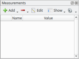
Measurements tool
To add a measurement use the Add dropdown and select ‘Define Measurement’. Which will give you an Add measurement selection box like shown below.
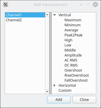
Measurements tool selection
Here you can select which channel you would like to make the measurement on as well as the type of measurement.
- Create a peak to peak voltage measurement for Channel 1 using the steps outlined above. Once created you should see that a measurement is being made on the incoming Channel 1 waveform with a reading about 2V. You can add as many measurements as you like.
Note:
These automatic measurements are only as good as the input waveform that you give them to do the calculations on. For example, If you are trying to obtain a voltage measurement and the signal is either really tiny on the screen or way to big for the screen (part of the waveform goes off the top of the display) the calculation will be made but could be incorrect. When making frequency or any measurement where the period of a cycle needs to be know, You need to make sure that more than a single cycle is shown.
2.6.5 Measuring Phase
Use the cursors on the scope to measure the relative phase between two signals.
Connect the Analog Discovery 2 to the computer and to your breadboard like you have done in the previous labs.
Open the ‘Waveforms’ program and make sure that it successfully connected to your Analog Discovery 2.
Connect the Wavegen 1 output to the Channel 1 input of the Scope and connect the Wavegen 2 output to the Channel 2 input of the Scope as shown in the circuit below.
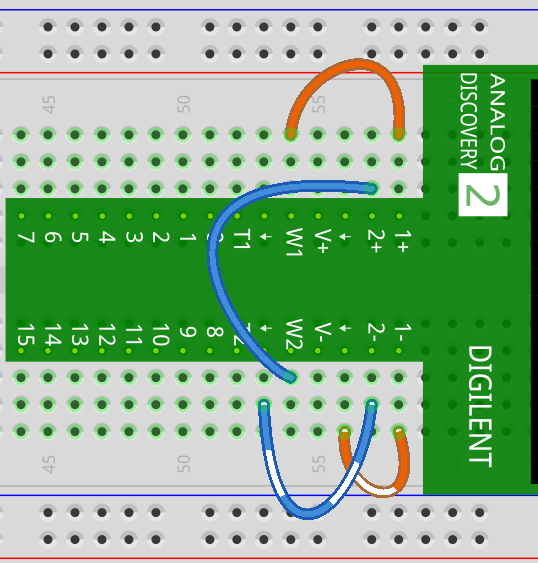
Both Wavegen to Scope channels
Using the Wavegen tool create 2 Sine waveforms both at 1kHz and 1VPeak with a phase shift from one another so we can learn how to measure the phase difference between those waveforms on the Scope.
- To do this, first make sure both channels (W1, W2) are displayed by using the Channels dropdown box as shown below.

Wavegen Channels dropdown
- Double check that both channels (W1, W2) are currently configured like the following:
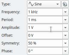
Wavegen Channels dropdown
Use the Channel 2 (W2) controls to change the Phase to 90°.
In the top toolbar in the dropdown to the right of the Channels dropdown you also need to select ‘Synchronized’ as shown below. This ensures that the phase between Channels 1 and 2 will output correctly.
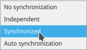
Wavegen Synchronized dropdown
- Click on the ‘Run All’ Button on the top toolbar to output the signals on the W1 and W2 pins on the Analog Discovery 2. Your Waveforms screen should now look like the following.
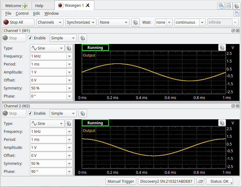
Wavegen running
With the Wavegen now running also open up the Scope tool in Waveforms and click on the ‘Run’ button. You should be able to see the 2 Wavegen outputs being measured on the Scopes display. Adjust the appropriate controls until you obtain a display like the one shown below.
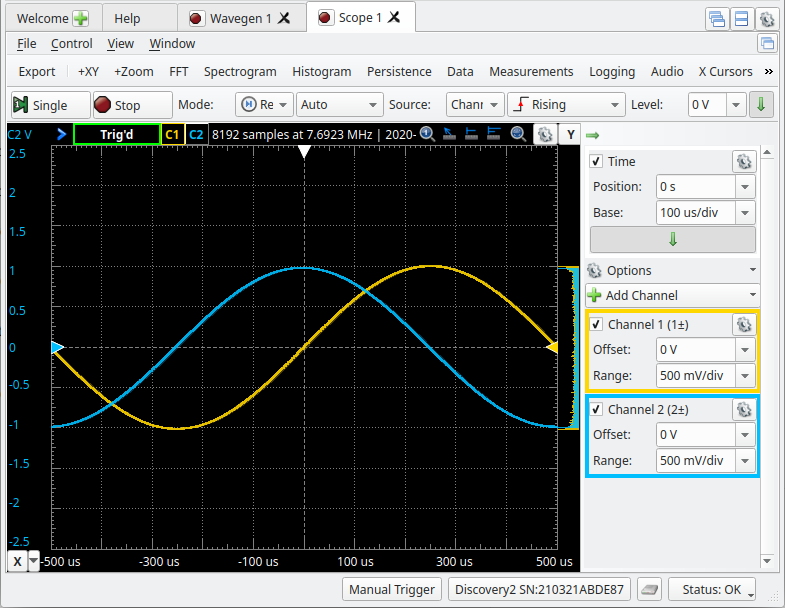
Scope running
As you can see above the blue waveform is “leading” the yellow waveform or the yellow is “lagging” the blue. To measure the phase difference between these 2 waveforms in time we can easily approximate this by counting the horizontal divisions from where the yellow crosses the 0V level to where the blue cross the 0V level. This is about 2.5 divisions and with a Base of 100us/div that works out to 250us. Knowing that the frequency of this waveform is 1kHz, the period is 1000us. So, to solve for the phase difference in degrees you simply need to take the measured 250us and divide by the period and then multiply by 360°. When doing this you notice that we get 90°, which is the same as the angle we put in to the Channel 2 Wavegen signal.
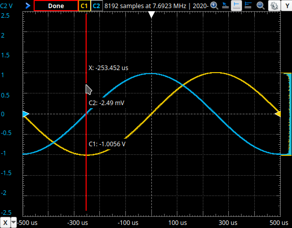
As the number of divisions don’t always work out so nicely as the example, you can either use the X Cursors tool located in the top toolbar or the Quick Measure tool I’m going to show here to make a quicker more accurate measurement. To activate the tool simple double click anywhere on the Scopes waveform display and your cursor will become a vertical red bar you can move around the display like the one shown below.
Scope quick measure
When you move the red cursor left and right on the display it will tell you the instantaneous voltage of both channels at the specific time that you have the cursor. First, find the closest time when the blue waveform (Ch2) is closest to 0V and click the mouse button. Second, move the cursor to the closest time when the yellow waveform (Ch1) is closest to 0V and click the mouse button again. Your display should now look similar to the one below.
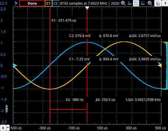
Scope quick measure
There is now a lot of information on the screen but the value that we are interested in is the ΔX. Which is the time between the 2 red cursors. On the display above this time is measured at 250.5us. Which closely matches what we measured when we simply counted the divisions. Below is the equation which turns this measured time into a phase value.
\[\phi = -(\frac{t_{Phase}}{period}) \times 360^{\circ}\]
Note:
When measuring the phase in time between two waveforms it is important to measure the time starting with the reference waveform to the waveform under test to obtain the correct sign. So, if the reference waveform is to the right of the waveform under test it is said to be “leading” and the sign will be negative. If the waveform under test is “lagging” the sign will then be positive. Recall that shifting left in time corresponds to a positive phase shift and shifting right to a negative. This effect is the opposite to the measurement. Therefore when converting from a phase in time to a phase in angle the sign needs to be switched. This is why there is a negative sign in the formula above.Note:
In a circuit it is convention to use the current relative to the voltage to decide if the circuit is leading or lagging. Therefore a circuit is lagging if the current lags the voltage and leading if the current leads the voltage.
2.7 Cleanup
Congratulations, you have completed the experimental part of this laboratory. If you are not continuing to work with the equipment please disconnect everything and put it away to prevent it from getting damaged.