Lab 2: Synchronous Machines
ECE332 - Electrical Machines
Electrical and Computer Engineering - University of Alberta
1 Introduction
1.1 Laboratory Goals
This lab will consider the operation of synchronous machines as both motors and generators. You will investigate a standalone synchronous generators voltage regulation depending on different load types. As well as a synchronous motors ability to consume or supply VARs to the power system regardless of the magnitude of load on the motor. Limits on the performance of the machines will also be explored. Note that the theory refers to round-rotor machines; saliency is beyond the scope of the course.
1.1.1 Circuits
Circuit 1A & 1B: Open-circuit speed and Open-circuit tests.
Circuit 2: Short-circuit Test.
Circuit 3A & 3B: Standalone generator load and unbalance test.
Circuit 4: Grid-connected Motor
1.2 Equipment
List of Equipment used for this Laboratory Experiment.
Power Supply – Model 8525-20
Data Acquisition and Control Interface (DACI) – Model 9063
2kW Three-phase Wound-field Synchronous Machine – Model 8507
Wiring Module for Synchronous Machine – Model 8508
2kW Four-quadrant Dynamometer – Model 8540
Safety banana Leads – 3 Colors, 3 Lengths
Computer running LVDAC-EMS software
Accessories – (USB cable, Barrel Power Cable)
2 Theory
Synchronous machines are similar to DC machines in that: they have a field winding and an armature winding; a dc current is passed through the field winding to produce flux; the flux from the field winding induces a voltage in the armature winding. However, unlike DC machines: the field winding is on the rotor and the armature winding is on the stator and the armature winding is an ac winding.
2.0.1 Armature Circuit
For the majority of the analysis of synchronous machine behaviour, we are only concerned with the armature circuit. We assume that there is a field winding that produces a flux which induces a voltage \(\overset{}{E}\) in the armature circuit. Note that \(\overset{}{E}\) is an ac phasor quantity, fully described as:
\[\overrightarrow{E} = \widehat{E}e^{j(\delta - \omega t)}\]
The rms magnitude of the induced voltage, E, is often referred to as the “excitation” and the phase angle, δ, is referred to as the “load angle”. The excitation of the armature is often dealt with as an independent variable. In reality, it is a function of the field winding, field circuit design and speed of rotation.
The steady-state behaviour of a synchronous machine may be described using the per-phase equivalent circuit models shown in Figure 1 and Figure 2. Notice that the only difference between the models is the definition of the direction of positive current flow: out of a generator and into a motor. The diagrams represent one phase of the machine, with V, E being phase voltages, Ra the armature resistance and XS the synchronous reactance.
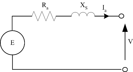
Figure 1: Generator per-phase equivalent circuit model

Figure 2: Motor per-phase equivalent circuit model
In many machines, it is reasonable to assume that XS >> Ra and resistance can be neglected. In this case, Figure 1 and Figure 2 can be replaced with Figure 3 and Figure 4.
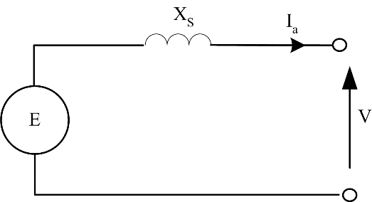
Figure 3: Simple generator per-phase circuit
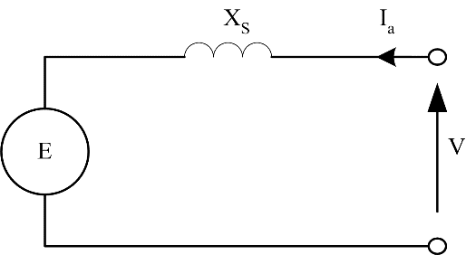
Figure 4: Simple motor per-phase circuit
2.0.2 Generating vs. Motoring
Viewing the circuit models, the only obvious distinction between motoring and generating is the defined direction for positive current. Writing down the voltage loop equation for a generator from Figure 1 results in equation (2).
\[\overrightarrow{E} = \overrightarrow{V} + j\overrightarrow{I_{a}}X_{s}\]
Writing down the voltage loop for a motor from Figure 2 results in equation (3).
\[\overrightarrow{V} = \overrightarrow{E} + j\overrightarrow{I_{s}}X_{s}\]
In the physical system, the distinction between motor and generator is related to power flow. If power flows from the mechanical system, through the machine to the electrical system, the machine is operating as a generator. If power flows from the electrical system, through the machine to the mechanical system, the machine is operating as a motor. To help understand the operation of a synchronous machine, it is usual to use phasor diagrams. The terminal voltage of the phase is defined as having zero phase angle, and the current, synchronous reactance voltage drop and excitation voltage are drawn relative to the terminal voltage. If positive power flows in the same direction as positive current then the phase angle of current relative to terminal voltage, θ, must be in the range:
\[- 90 \leq \theta \leq 90\]
Constructing a phasor diagram, it becomes clear that
\(\overrightarrow{E}\) leads \(\overrightarrow{V}\) in a generator, and
\(\overrightarrow{E}\) lags \(\overrightarrow{V}\) in a motor
The four basic shapes of the phasor diagrams for the per-phase equivalent circuits shown in Figure 3 and Figure 4 are shown in Figure 5, Figure 6, Figure 7 and Figure 8. It can be seen that the terminal power factor is a function of the magnitude of the excitation. If |E|>|V| in a generator, then for equation (2) to hold, the power factor must be lagging. Similarly, if |E|<|V| then the power factor must be leading
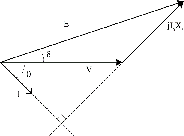
Figure 5: Over-excited generator - (lagging PF)
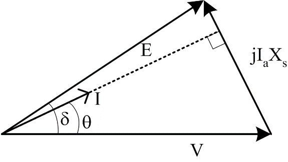
Figure 6: Under-excited generator - (leading PF)
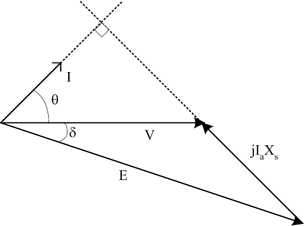
Figure 7: Over-excited motor - (leading PF)
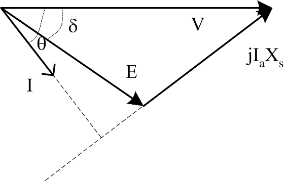
Figure 8: Under-excited motor - (lagging PF)
For a motor, it can be seen that for equation (3) to hold, an over-excited motor must have a leading power factor. From these observations, and knowledge of a typical power system, one can state that the majority of synchronous machines will be operated with |E|>|V|. (Most loads on the power system are lagging, so generators must generate the VARs required by the system, also operating at lagging power factor. Most times when a synchronous motor is used, it is operated at leading power factor to help improve the overall power factor at a site.) Note that in this lab when the synchronous machine is grid connected, we will assume that the supply is an infinite bus: |V| is constant, f is constant.
2.0.3 Field Circuit
The field of synchronous machine can be created either by a winding or a permanent magnet. Permanent magnet machines have typically been small motors, although large multi-MW machines are currently under development for military applications. In typical synchronous generators and medium-large size synchronous motors, the rotor field is created using a DC field winding. Unlike a DC machine field winding, the field winding is rotating at synchronous speed; this creates the difficulty of how to create the rotor DC field current. Two possible options are available:
Use slip rings and carbon brushes to supply the DC current from an external source.
Generate an ac voltage on the shaft by using an additional stationary field winding and rotating conductors. Then rectify the induced ac voltage over the rotating conductors to DC, with diodes mounted on the rotor. No slip rings and brushes are needed for this case.
The first option is often popular as the initial capital cost is lower. This is offset by higher operating costs as maintenance is required on the brushes and slip rings. The second option is often used in larger machines. A small ac generator called a brushless exciter has its armature circuit mounted on the shaft of the rotor, and its dc field circuit mounted on the stator. The generated AC current is then rectified directly on the rotor using a 3-phase rectifier.
In this lab manual If represents the DC currents in different windings depending on the type of exciter. For synchronous machines with brushes, If represents the rotor field current supplied directly from an external source. For brushless synchronous machines, If represents the DC current in the field circuit mounted on the stator.
2.0.4 Torque and Power
Equations to approximate power and torque can be found from the simplified phasor diagram. It can be seen in Figure 9 that the load angle and power factor angle are related by:
\[E\sin{\delta = I_{a}X_{s}\cos\theta}\]
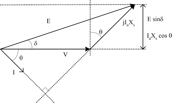
Figure 9: Phasor diagram angles
Using the definition for voltamps and power in a 3-phase system:
\[S = 3VI\]
\[P = S\cos\theta\]
Where V and I represent phase quantities. Substituting equation (5) into equations (6) and (7) gives:
\[P = \frac{3VE}{X_{s}}\sin\delta\]
Using the mechanical power equation
\[P_{\text{mech}} = \tau\omega_{m}\]
And noting that in a synchronous machine mechanical speed equals synchronous speed,
\[\omega_{m} = \omega_{s} = \frac{4\pi f}{p}\]
Results in the torque equation
\[\tau = \frac{3VE}{X_{s}\omega_{s}}\sin\delta\]
Note that f is frequency in Hz, p is the number of poles in the machine. Using equation (8) and the phasor diagram of Figure 9 it can be scaled to give power and VARs, shown in Figure 10.
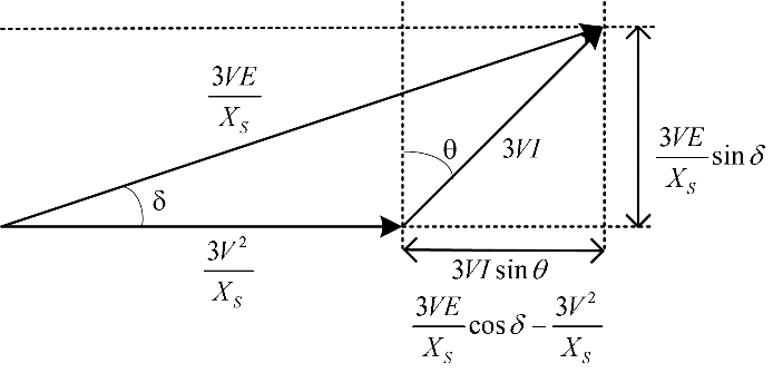
Figure 10: Phasor Diagram of Power
It can be seen in Figure 10 that for a generator.
\[Q = 3VI\sin\theta\]
\[Q = \frac{3VE}{X_{s}}\cos{\delta - \frac{3V^{2}}{X_{s}}}\]
For a motor, due to the change in direction of positive current,
\[Q = \frac{3V^{2}}{X_{s}} - \frac{3VE}{X_{s}}\cos\delta\]
Re-plotting the data from Figure 10 to plot power on the positive x-axis and VARs on the positive y-axis, it is possible to plot the operating chart of a synchronous machine, shown in Figure 11.
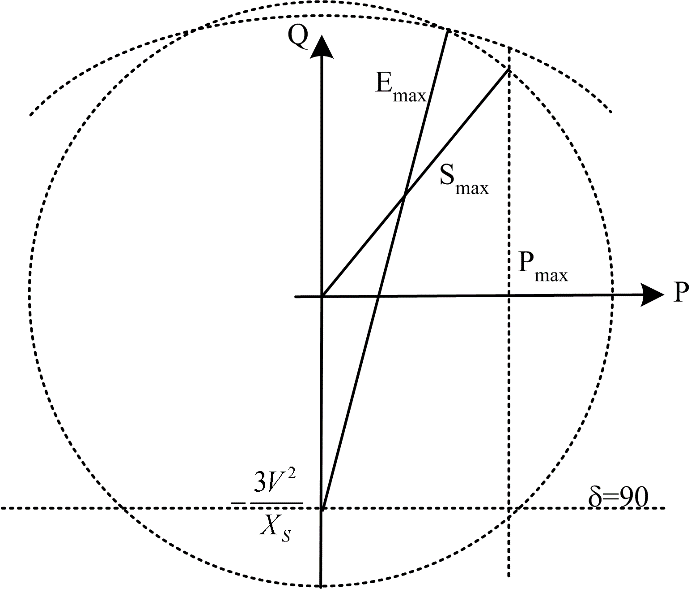
Figure 11: Synchronous Machine Operating Chart
A machine can operate anywhere within the following limits:
Stator heating limit; Smax. Set by the maximum allowable armature current
Rotor heating limit; Emax. Set by the maximum allowable field winding current.
Prime mover limit; Pmax. The maximum power available from the mechanical system.
Static stability limit, δ=90°. The limiting case of equation (8).
Finally, the case where the armature resistance is not negligible must be considered. In this case, the terminal electrical power is given by
\[P_{t} = 3VI\cos\theta\]
or
\[P_{t} = \sqrt{3}V_{\text{LL}}I_{L}\cos\theta\]
And the armature losses are given by
\[P_{\text{scl}} = 3I_{a}^{2}R_{a}\]
The relationship between electrical terminal power and the mechanical power depends on whether the machine is a motor or generator. For a generator:
\[P_{\text{mech}} = P_{t} + P_{\text{scl}}\]
For a motor:
\[P_{\text{mech}} = P_{t} - P_{\text{scl}}\]
Torque can be found from the mechanical power using equation (9).
2.0.5 Parallel Operation of Synchronous Generators
The majority of synchronous generators are operated in parallel with other generators. Most generators are connected to a power grid. Exceptions to grid connection include emergency generators and remote sites (including communities in the north, logging and drilling camps), though these situations often have a number of generators in parallel. When connecting generators to a system with an existing voltage certain conditions must be fulfilled:
The RMS line voltages must be equal.
The phase sequences should be consistent.
The connection must be made at or near an instant when the two voltages are in phase.
The generator frequency must be slightly higher or lower than the system frequency.
The simplest method to meet these conditions is to use synchronization lamps connected across the contactor, as shown in Figure 12:

Figure 12: Synchronization Circuit
Depending on the state of the lamps, differences in the voltage conditions across the contacts can be determined.
The possible voltage conditions and lamp states are listed below.
All conditions are met. The lamps will flash in union at a very low frequency equal to the difference between the generator and system frequencies.
Phase sequencing is incorrect. The lamps will flash at different times. This can be corrected by interchanging two of the machine phases.
There is a big difference between the generator and system frequencies. The lamps will flash in unison at a high frequency. In this case, adjust the speed of the generator to reduce the frequency of the lamps.
Voltage magnitudes are different. The lamps will glow steadily. The brightness of the lamps is a function of the voltage difference. Increase or decrease the excitation to reduce the intensity of the lamps.
Phase angles are not equal. The lamps will glow steadily. It is unlikely that the generator and system will have exactly the same frequency and constant phase angle error.
2.0.6 Starting a Synchronous Motor
Synchronous machines only produce torque at synchronous speed. Generators are usually brought to synchronous speed by the mechanical system, but starting motors is more challenging. Many synchronous motors are constructed with an induction cage on the rotor. This allows the motor to start from standstill and accelerate to synchronous speed. Once the motor is at synchronous speed, the field winding can be turned on and the machine acts like a synchronous motor. Other options include placing a small induction motor on the same shaft as the synchronous machine. The induction machine accelerates the synchronous machine to synchronous speed with no load attached. Once at synchronous speed, the synchronous machine is energised and a load applied via a mechanical clutch. A final option involves using a variable frequency supply to slowly accelerate the machine to the desired operating synchronous speed.
2.0.7 Open and Short Circuit Tests
The accurate determination of synchronous reactance is non-trivial. Synchronous reactance depends not only on field current, but also load angle, armature current and armature reactance. However, if we assume that it is possible to linearize the system about the rated voltage, and that armature reaction always opposes the rotor magnetic field, then it is possible to derive an estimate of the synchronous reactance based on open circuit and short circuit tests.
During an open circuit test, the machine operates at synchronous speed and the variation of line-line voltage with field current is recorded. During a short circuit test, the terminals are short circuited and the variation of short circuit armature current with field current is recorded. Typical plots of o/c voltage and s/c current are shown in Figure 13.
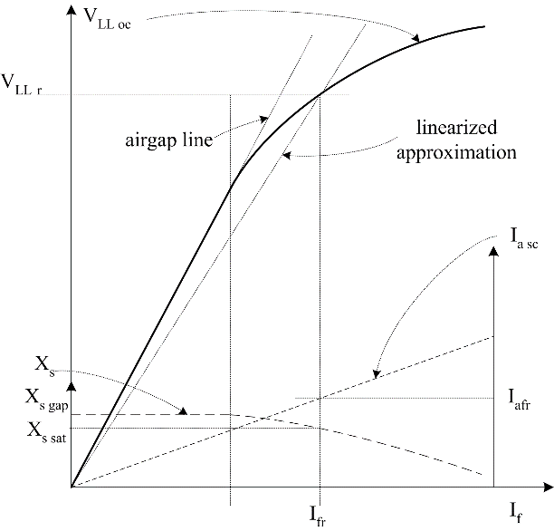
Figure 13: Synchronous Machine Open and Short Circuit Test Data
Open circuit phase voltage (also the excitation) is given by:
\[E = \sqrt{2}\pi N_{c}\widehat{\phi}f\]
At lower field current levels, the field current-flux relationship is linear and terminal voltage rises linearly with field current. As the field current increases during the open circuit test, saturation occurs and the incremental rate of change of voltage with field current is reduced. During the short circuit test, the flux produced by the armature winding acts against the field winding flux, reducing the total flux in the machine and preventing saturation. As a result, short circuit armature current increases linearly with field current. Now, during the short circuit test, the per phase equivalent circuit model may be drawn as in Figure 14.
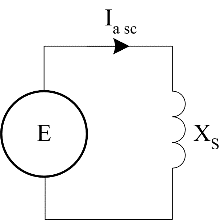
Figure 14: Short circuit test equivalent circuit model
It can be seen that:
\[X_{s} = \frac{E}{I_{a\ (sc)}}\]
More strictly:
\[X_{s}\left( I_{f} \right) = \frac{E_{(oc)}(I_{f})}{I_{a\ (sc)}(I_{f})}\]
A plot of synchronous reactance as a function of field current is shown on the graph in Figure 13. It can be seen that even using these simple assumptions synchronous reactance is nonlinear. An approximation is possible if the system is linearized about the rated terminal voltage for the machine. To find XSsat as shown in Figure 13, the following procedure is used:
Find the field current that will produce rated open circuit terminal voltage, Ifr
Find the short circuit armature current Ia(fr) that corresponds to the field current Ifr.
Find the reactance given by
\[X_{S_{\text{sat}}} = \frac{V_{\text{rated}}}{I_{a\ (fr)}}\]
It should be noted that this reactance is an approximation. It is based on the assumption that armature reaction opposes rotor flux. As a result, the approximation should be best when generating with a lagging power factor.
3 Pre-lab
The Pre-lab is to be completed and handed-in at the beginning of your schedule lab session. You will not be allowed to participate in the Laboratory Experiments until your Pre-lab has been completed.
3.1 Pre-lab Reading
Familiarize yourself with the lab procedures and requirements by reading through the lab manual.
Familiarize yourself with the Safety Rules as well as the Equipment and Software used in the third Laboratory by viewing the information on the laboratory webpage below:
Note the equipment datasheets can be located at the bottom each page.
To access the webpage, you need to be logged-in with your CCID.
Re-watch the ‘General Lab Safety’ video available on eClass.
Review Synchronous Machine theory.
Have at least, the “ECE332 - Lab 2 – Sign-off” sheet printed off before coming to the lab.
3.2 Pre-lab Questions
The information for questions 1-8 can be found either in the Lab 2 manual or on the webpage and datasheets mentioned above. Answer the questions on a separate piece of paper to be handed-in at the beginning of your schedule lab session (Show all of your work). Make sure you clearly put your name, student ID number, CCID and your lab section at the top of the page.
What are the goals of this lab?
In the open circuit tests, what do you use to set the speed of the synchronous machine?
During the open and short circuit tests, do you supply electrical power to the stator winding of the synchronous machine?
What range of stator currents do you expect in the short circuit test? With this expected range, what range should you use on the Data Acquisition and Control Interface to measure these currents?
How is the stand-alone synchronous generator loaded?
How is the grid-connected synchronous motor loaded?
How is the reactive power flow controlled in the grid-connected synchronous motor?
Does an over-excited grid connected synchronous motor operate with leading or lagging power factor?
4 Lab Procedure
4.1 Startup
Login to the computer at your station. Use your CCID and password.
Connect and power the Data Acquisition and Control Interface (DACI) and launch the LVDAC-EMS software.
Make sure you use 120V, 60Hz for your system voltage and frequency
Make sure the “Work in standalone mode” is unchecked.
To setup the machines for this experiment if not already completed for the station you are working at:
Couple the synchronous machine to the 4-quadrant dynamometer using the rubber coupling.
Plug in 4-quadrant dynamometer in to the available 3 phase receptacle.
Attach the synchronous machine cable bundle to the back of wiring module using the provided connector.
4.2 Circuit 1 - Open-Circuit Tests
There are 2 separate open-circuit tests. In these tests you use another device to make the shaft rotate in our case the 4-quadrant dynamometer or (dyno). With the shaft rotating and adjusting the rotor field current, which controls the strength of the magnetic field on the rotor, we measure the effect that speed has on the stator voltage in the first test and then how the rotor current effects the voltage in the second test.
4.2.1 Circuit Setup
Connect the circuit shown in Figure 15.
Connect the main variable DC supply to the synchronous machine rotor circuit.
Use E4 and I4 to measure both the voltage across and current in the rotor field circuit
Connect the stator of the motor in a wye by shorting terminals 4, 5 and 6 together on the synchronous machine panel.
Use E1 to measure the open circuit voltage of the stator.
Make sure that the rotor field circuit switch on the synchronous machine panel is in the closed/up/1 position.
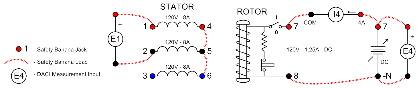
Figure 15: Open-circuit Test Circuit
4.2.2 Instrument Setup
- Setup the Metering Instrument as follow in Table 1. Open-circuit Tests Table 1.
| Meter | Description | Type | Input/Function | Mode |
|---|---|---|---|---|
| M1 | A-B Line-to-line stator voltage | Voltage | E1 | AC |
| M4 | DC rotor field voltage | Voltage | E4 | DC |
| M10 | DC rotor field current (4A) | Current | I4 | DC |
- Setup the Data Table to record the data from the Metering Instrument.
4.2.3 Circuit 1A - Speed Test Results
When you think your circuit and instrumentation is setup correctly get an instructor or TA to verify it before you apply power.
Turn on the 4 quadrant dynamometer (dyno) by turning on the switch next to the embedded vector drive on the dyno. Once it powers up, enter “Speed Mode” by pressing the touch screen button.
Press “Fwd” on the dyno display to start the dyno. Its speed should currently be set to 0rpm and will not be rotating but you should be able to hear the power electronics buzzing. Using the arrows on the display increase the dyno speed to 1800rpm (The synchronous machines rated speed).
Ensure the main power supply control variac is currently set at 0%.
Apply power by using the main power switch, L1, L2 and L3 should light up to indicate power.
Increase the rotor field current by adjusting the main power supply control variac until you get the rated synchronous machines line-line voltage (208V) at its armature terminals shown on M1 of the Metering Instrument. Make a note of the main power supply control variac and rotor field current setting at this point for use later in the lab. (_______%, _______Amp)
Record the data at this set point using the Data Table.
By either using the arrows on the dyno’s display or by clicking on the displayed speed value and entering in a desired speed. Reduce the speed by 200rpm at a time recording the Data Table at each step from 1800rpm down to 200rpm. Make sure that you keep the rotor field current constant for the entire test.
Once you have captured all the speed settings above, export the Data Table to a .csv or .dat file. Save the file somewhere you will have access to after the Laboratory.
Decrease the speed down to zero and press stop to turn off the dyno. Decrease the main power supply variac back to zero and turn off the power supply.
4.2.4 Circuit 1B - Open Circuit Test Results
Again use the dyno to get the shaft up to rated speed by entering “Speed Mode” and pressing “Fwd” on the dyno display and entering a speed of 1800rpm.
Ensure the power supply variac is currently set at 0%.
Apply power by using the main power switch, L1, L2 and L3 should light up to indicate power.
Slowly Increase the rotor field current by increasing the main power supply control variac and record the Data Table at 30 V increments of the open circuit armature line-to-line voltage indicated on M1, from 30 V to 270 V.
Once you have captured the data at of the all the voltage settings above, export the Data Table to a .csv or .dat file. Save the file somewhere you will have access to after the Laboratory.
Decrease the speed down to zero and press stop to turn off the dyno. Decrease the main power supply variac back to zero and turn off the power supply.
Get an instructor or TA to view your results for both test 1A and 1B and get them to sign off on your results sheet.
4.3 Circuit 2 - Short-Circuit Test
The short circuit test is very similar to the open circuit test except that you short the stator armature output voltage and measure the resulting armature currents. Using the results of both tests allows you to calculate the synchronous reactance at different values of field current.
4.3.1 Circuit Setup
Connect the circuit shown in Figure 16. Short-circuit.
Leave the rotor field circuit connected as before in circuit 1.
With the Stator circuit still connected in a WYE, short circuit the armature output by using I1 on the 40 Amp scale between terminals 1 and 2, and shorting terminals 2 and 3 with a safety banana lead.
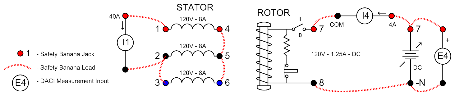
Figure 16: Short-circuit Test Circuit
4.3.2 Instrument Setup
Setup the Metering Instrument as shown in Table 2.
- Make sure in the LVDAQ-EMS software that you also set the current range for I1 to be 40Amps under the “Data Acquisition and Control Settings” sidebar.
| Meter | Description | Type | Input/Function | Mode |
|---|---|---|---|---|
| M4 | DC rotor field voltage | Voltage | E4 | DC |
| M7 | Stator short-circuit current (40A) | Current | I1 | AC |
| M10 | DC rotor field current (4A) | Current | I4 | DC |
Table: Table 2. Short-circuit Test (Meter Setup)
- Refresh the Data Table Setup to Record the new Metering Instrument setup.
4.3.3 Results
Again use the dyno to get the shaft up to rated speed by entering “Speed Mode” and pressing “Fwd” on the dyno display and entering a speed of 1800rpm.
Ensure the main power supply control variac is currently set at 0%.
Apply power by using the main power switch, L1, L2 and L3 should light up to indicate power.
Slowly Increase the rotor field current by increasing the main power supply control variac and record the Data Table at 1 amp increments of the short circuit armature current indicated on M7, from 1A to 8A.
Once you have captured all the speed settings above, export the Data Table to a .csv or .dat file. Save the file somewhere you will have access to after the Laboratory.
Decrease the speed down to zero and press stop to turn off the dyno. Decrease the main power supply variac back to zero and turn off the power supply.
Get an instructor or TA to view your results and sign off on your results sheet.
4.4 Circuit 3 - Standalone Generator Load Test
In this test you will use the 4 quadrant dynamometer as a prime mover to get the synchronous machine up to synchronous speed. You will then use the wye connected 3ph synchronous machine as a generator to supply power to either a resistive, inductive or capacitive load to see how the generator is effected by different load types. In the second part of this test you will see how an unbalanced load effects the output voltage of a synchronous generator.
4.4.1 Circuit Setup
Connect the circuit shown in Figure 17.
Leave the rotor circuit the same as the previous circuits.
Connect the R, L and C Load Boxes in a 3ph parallel wye configuration as shown.
Use I1, I2 and I3 to measure the 3 stator phase currents. Use the 4A setting for each of these.
Use E1, E2 and E3 to measure the 3 stator line-to-line voltages, labels A, B and C are used to show the connections.
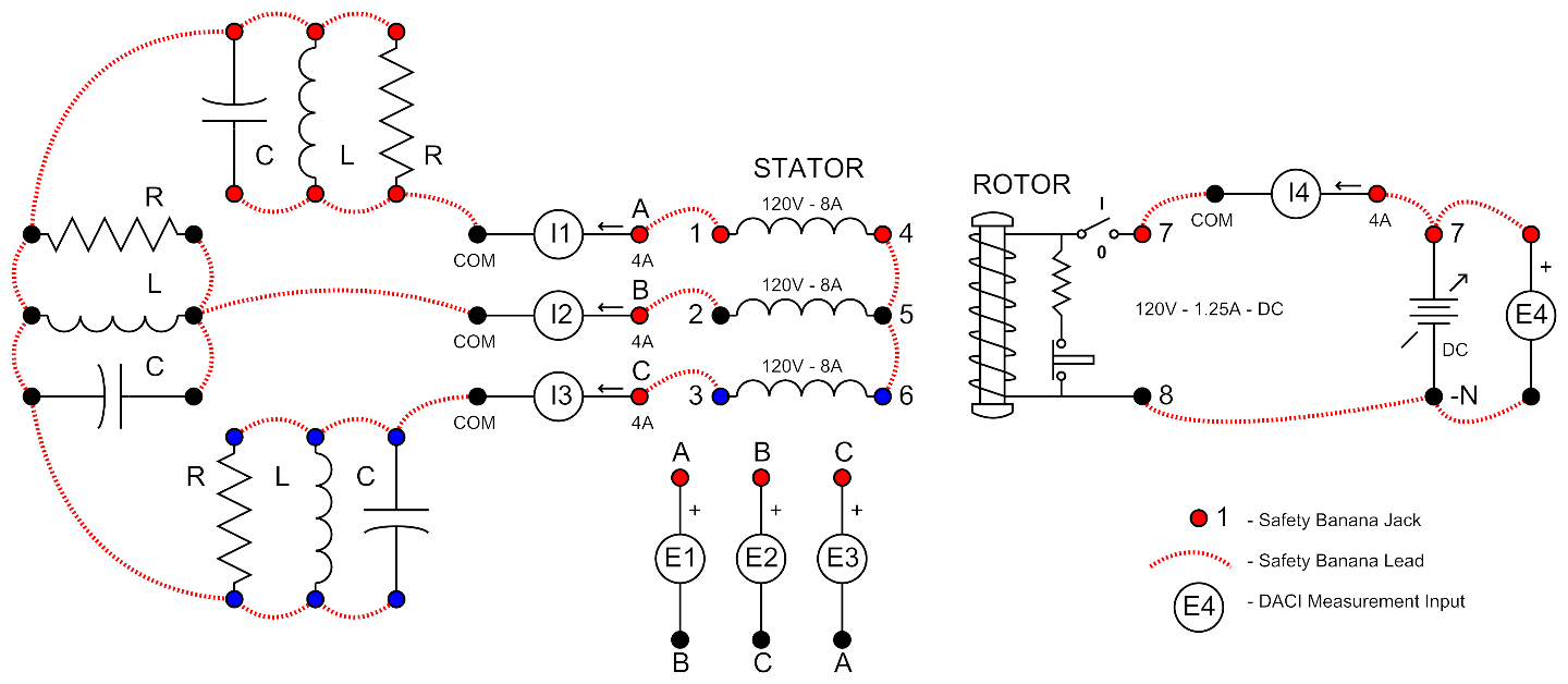
Figure 17: Standalone Generator Circuit
4.4.2 Instrument Setup
Setup the Metering Instrument as shown in Table 4.
- Make sure in the LVDAQ-EMS software that you also set the appropriate current scales for each current meter under the “Data Acquisition and Control Settings” sidebar.
| Meter | Description | Type | Input/Function | Mode |
|---|---|---|---|---|
| M1 | A-B line-to-line stator voltage | Voltage | E1 | AC |
| M2 | B-C line-to-line stator voltage | Voltage | E2 | AC |
| M3 | C-A line-to-line stator voltage | Voltage | E3 | AC |
| M4 | DC rotor field voltage | Voltage | E4 | DC |
| M7 | Phase A stator current (4A) | Current | I1 | AC |
| M8 | Phase B stator current (4A) | Current | I2 | AC |
| M9 | Phase C stator current (4A) | Current | I3 | AC |
| M10 | DC rotor field current (4A) | Current | I4 | DC |
- Refresh the Data Table setup so the new Metering Instrument setup can be recorded.
4.4.3 Circuit 3A - Standalone Generator Load Test Results
Again use the Dyno to get the shaft up to rated speed by entering “Speed Mode” and pressing “Fwd” on the Dyno Display and entering a speed of 1800rpm.
Ensure the main power supply control variac is currently set at 0%.
Start with all the resistor, inductor and capacitor load switches in the off/down position.
Apply power by using the main power switch, L1, L2 and L3 should light up to indicate power.
Increase the field current by increasing the main power supply variac until you get an A-B line-to line stator voltage of approximately 208V. Do not adjust the field current for the rest of this experiment.
The standalone synchronous generator is now running un-loaded, record this point in Data Table.
Turn on all 9 of the switches for the resistor load box to load the machine as much as possible with the equipment available. Note that this is actually about a quarter of rated full load of the generator, but is sufficient to show the effect of different load types on the synchronous generator. Record this set point in the Data Table for a resistive load.
Turn off all of the switches in the resistor load box and turn on all of the switches in the inductive load box. Record this set point for an inductive load.
Continue by turning off all the switches in the inductive load box and turning on all of the switches in the capacitive load box. Record this set point for a capacitive load.
Once you have captured all 4 of the required set points above, export the Data Table to a .csv or .dat file. Save the file somewhere you will have access to after the Laboratory.
Turn off all of the switches in the capacitive load box but leave everything else and continue on with the next test.
4.4.4 Circuit 3B - Standalone Generator Unbalanced Test Results
Clear the Data Table.
Make sure all resistive, inductive and capacitive load switches are off, in the down position.
Record the current Metering Instrument readings for the unloaded generator into the Data Table.
Turn on the resistor and inductor switches in only 2 of the phases and keep the third phase with all of the switches off to create an unbalanced load on the generator.
Record this unbalanced load condition in the Data Table.
Turn off all of the load switches, return the main power supply control variac to 0% and turn off the main power supply, reduce the speed of the dyno to 0rpm and press “Stop”.
Get an instructor or TA to view your results for both test 3A and 3B and get them to sign off on your results sheet.
4.5 Circuit 4 - Grid Connected Motor
In this test you will use the synchronous motors squirrel cage to get the motor connected to the grid. Once connected you will load the motor and see how the field voltage effects the motors reactive power consumption.
4.5.1 Circuit Setup
- Connect the circuit shown in Figure 18.
Leave the rotor field circuit connected as before in circuits 1 and 2.
Connect the Fixed AC Supply to the WYE-connected Stator circuit.
Use E1, I1, E2 and I2 metering inputs connected as the 2 wattmeter method, make sure you use the 40 amp input scale for the currents.
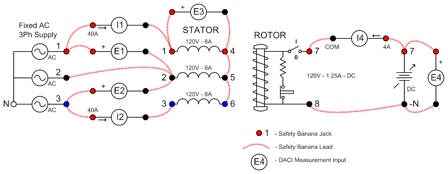
Figure 18: Grid-connected Motor Circuit
4.5.2 Instrument Setup
Setup the Metering Instrument as shown in Table 4.
- Make sure in the LVDAQ-EMS software that you also set the appropriate current scales for each current meter under the “Data Acquisition and Control Settings” sidebar.
| Meter | Description | Type | Input/Function | Mode |
|---|---|---|---|---|
| M1 | AB line-to-line stator voltage | Voltage | E1 | AC |
| M2 | CB line-to-line stator voltage | Voltage | E2 | AC |
| M3 | Phase A stator voltage | Voltage | E3 | AC |
| M4 | Rotor field voltage | Voltage | E4 | DC |
| M7 | Phase A stator current (40A) | Current | I1 | AC |
| M8 | Phase C stator current (40A) | Current | I2 | AC |
| M10 | Rotor field current (4A) | Current | I4 | DC |
| M13 | 3Ph input power | Power | PQS1 + PQS2 | P |
| M14 | 3Ph input reactive power | Power | PQS1 + PQS2 | Q |
| M15 | 3Ph input apparent power | Power | PQS1 + PQS2 | S |
| M16 | Input power factor | Power Factor | PF (EI1, EI2) | True |
Refresh the Data Table Setup to Record the new Metering Instrument setup.
Launch the Phasor Analyzer and plot both the Phase A stator current “I1” and the Phase A stator voltage “E3”. Use E3 as the Reference. You may need to adjust the scales as necessary.
4.5.3 Motor Starting
This synchronous machine includes a squirrel-cage induction winding on its rotor for the specific use of motor starting. In order for the machine to start as an induction motor no field current should be present. On the rotor circuit on the synchronous machine wiring panel is a switch with 0/I marking above and below the switch, this switch is open when the switch is down or in the 0 position and therefore no rotor current will flow and short when the switch is up or in the 1 position allowing rotor current to flow. When a 3ph supply is connected to the stator the machine will start-up using the squirrel-cage and rotate close enough to synchronous speed that when a rotor field current is supplied it will automatically lock in to synchronous speed.
Make sure the Rotor field circuit switch is in the open/down/0 position.
Make sure that the dyno is currently off.
Before turning on the power supply increase the main control variac to the value noted at in circuit 1.
Turn on the power supply and the machine will speed up quickly to something close to synchronous speed.
Once the machine reaches a steady-state speed the Rotor field circuit switch can be switched to the short/up/1 position.
The Synchronous machine should now be synchronized to the grid.
4.5.4 Results
On the Dyno enter “Torque Mode”, press “Start” and increase the torque on the dyno to 3.56Nm.
If you take a minute and adjust the rotor field current by adjusting the main control variac you will notice what occurs with the synchronous machine operation. While doing this watch the stator currents that they don’t exceed their maximum rating of 6.8 Amps while running as a motor.
Adjust the rotor field current until you get an under-excited power factor of 0.5 and record a new Data Table at this set point. From this point, increase the rotor field current until you also get under-excited power factors of 0.6, 0.7, 0.8 and 0.9 recording the Data Table at each of these set points. If you continue to increase the rotor field current you will get something close to unity power factor, record a data point at close to a power factor of 1 as you can get. If you continue to further increase the rotor field current the machine is now over-excited and the power factor begins to drop. Record data points for over-excited power factors of 0.9, 0.8, 0.7, 0.6 and 0.5.
Once you have captured all the power factor points above, export the Data Table to a .csv or .dat file. Save the file somewhere you will have access to after the Laboratory.
Decrease the torque down to zero and press stop to turn off the dyno. Turn off the main power supply to stop the motor, the motor will coast to stop and can take about 1 minute or so. Decrease the main power supply variac back to zero.
Get an instructor or TA to view your results and sign off on your results sheet.
4.6 Clean Up
Verify your results with an instructor or TA to show that you have completed everything.
Cleanup your station, everything should be returned to where you got it from.
Once everything is completed and tidy get a signature on your Results page before you leave.
5 Postlab
5.1 Results Spreadsheet
Once you have all the required measurements recorded in your .dat or .csv files. On the ECE332 eClass page under Lab 4, download the spreadsheet called “ECE332 – Lab 4 – Results.xlsx”. Import or Copy and Paste your results from the .dat or .csv files into the provided spreadsheet. It will automatically calculate all the required information and plot the required graphs. Print a copy of the spreadsheet tabs Results and Graphs to hand in with your report.
5.2 Sample Calculations
The following sample calculations must be handed in with your results. Use the methods that are discussed in the lab manual. (Show all your work):
Calculate Xs (sat) for a VLLoc = 210V. You may need linear interpolation.
Calculate the Voltage Regulation (VR) for the capacitive load case.
Calculate the synchronous reactance (XS) phase angle (θ), load angle (δ) and excitation (E) for the grid connected synchronous motor at the operating point at 0.7 power factor over-excited. You may need linear interpolation to calculate Xs for this question.
Draw the phasor diagrams for the above case. Include Ia, V, E, IaXs, δ and θ in your drawings.
5.3 Questions
Answer the following questions to hand in with your lab report.
Considering the plot of open circuit voltage vs. speed, is the machine excited using brushes or a brushless exciter? Explain your choice.
Why does the rotor field current magnitude effect the synchronous reactance?
Look at the Short Circuit Current vs. Field Current graph. Why is the relationship between short circuit current and field current linear?
Why does the Standalone generator experience a stator voltage increase when loaded with a capacitor?
With a standalone generator what can be adjusted to compensate the change in stator output voltage when different balanced RLC load configurations are connected? Would this solution also be effective for an unbalanced load? Explain your answer.
In the grid connected motor experiment explain why the real output mechanical power is fixed?
Explain the shape of both the grid connected motor armature current vs. field current and armature current vs. reactive power plots.
Explain the shapes of the grid connected motor E and I loci.
Hint
For question 7 and 8: You may need to use phasor diagrams and relevant equations to analyze the trends of those curves.