Lab 1: DC Motors
ECE332 - Electrical Machines
Electrical and Computer Engineering - University of Alberta
1 Introduction
1.1 Laboratory Goals
The objective of this laboratory is to determine the operating characteristics of two types of DC motor: separately excited and series. For the first circuit you will apply a DC voltage and current to the different windings of the DC Motor so the winding resistances can be determined.
1.1.1 Circuits
Circuit 1: DC Resistance Measurements.
Circuit 2: No-load Separately Excited Tests.
Circuit 3: Separately Excited Load Test.
Circuit 4: Series Connected Load Test.
1.2 Equipment
List of Equipment used for this Laboratory Experiment.
Power Supply – Model 8525-20
Data Acquisition and Control Interface (DACI) – Model 9063
DC Motor/Generator – Model 8211-00
Electrodynamometer – Model 8911-10
Digital Tachometer – Model HT-341
Safety banana Leads – 3 Colors, 3 Lengths
Computer running LVDAC-EMS software
Accessories – (USB cable, Barrel Power Cable)
2 Theory
2.1 DC Motors
All DC motors have the same fundamental topology. There is a stationary part, the stator, which carries a field winding. The field winding is designed to create a stationary magnetic field which passes through the rotating part of the motor, the rotor. The rotor carries an armature winding. The armature winding is connected through moving contacts (slip rings and brushes) to an external voltage supply. The power flow in the armature winding is relatively high, while the power in the field winding circuit is much lower. The different techniques for supplying power to the field winding result in different types of motor with different characteristics. (The armature design is similar for all types of DC motor). All DC motors have the same two fundamental equations:
\[E_{a} = k\phi\omega_{m}\]
\[\tau_{\text{dev}} = k\phi I_{a}\]
Where:
Ea and Ia are the armature Voltage and Current.
ωm is the mechanical speed, in radians per second, ωm is related to nm, the speed in revolutions per minute (rpm) by:
k is a constant depending on the armature design,
τdev is the electromagnetic torque developed,
φ is the flux linking the armature, produced by the field winding.
The developed power can be found by rearranging equations (1) and (2):
\[P_{\text{dev}} = \tau_{\text{dev}}\omega_{m} = E_{a}I_{a}\]
Other DC machine equations are dependent on how the field is connected. A few different DC machine connections are:
Separately Excited
Shunt Excited
Series Excited
Compound
Permanent Magnet
The Separately Excited and Series DC Machine will be the focus in this lab.
2.2 Separately Excited
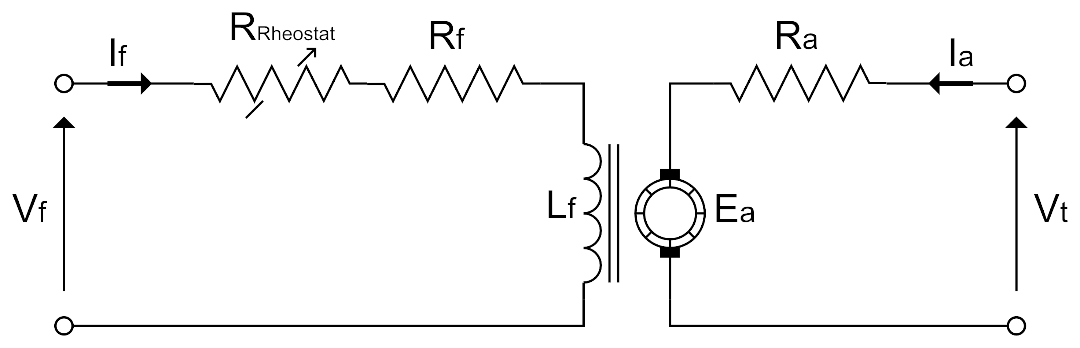
Figure 1: Separately Excited DC Motor Equivalent Circuit
A separately excited motor has a field winding which is supplied independently from the armature supply. Shown in Figure 1, the equivalent circuit model has two distinct circuits. Vf and If are the field winding voltage and current, respectively. Lf is an ideal field inductance and has zero voltage drop in steady state. The total field circuit resistance RF is made up of the actual winding resistance, Rf and any adjustable resistance in the field circuit, usually a Rheostat.
\[R_{F} = R_{f} + R_{\text{Rheostat}}\]
The flux in the machine is controlled by changing the field current. When separately excited it is usually controlled by adjusting either the field voltage or field resistance as shown in equation (5). However, due to saturation, the relationship between the field current and flux is nonlinear.
\[I_{f} = \frac{V_{f}}{R_{F}}\]
For separately excited the terminal voltage is defined as:
\[V_{t} = E_{a} + I_{a}R_{a}\] Substituting equations (1) and (2) into equation (6) we obtain the torque-speed characteristic of a separately excited DC motor:
\[\omega_{m} = \frac{V_{t}}{\text{kϕ}} - \frac{R_{a}}{{(k\phi)}^{2}}\tau_{\text{dev}}\]
As torque increases, the speed decreases. The equation becomes non-linear if either Vt, Ra, or flux changes. At high armature currents, the armature field can act to reduce the total flux from the field winding. This is called armature reaction. Sometimes compensating windings are introduced to counteract armature reaction.
There are 4 possible methods to control the speed of a separately excited DC motor:
Field voltage control, altering If and therefore changing φ in the machine;
Field resistance control, altering If and also changing φ in the machine;
Terminal voltage control, which changes the speed required to generate the steady state Back-EMF (Ea)
Additional resistance in series with the armature, effectively increasing Ra.
Options 1 and 2 control the motor by means of field winding current and flux. Options 3 and 4 control the motor by means of the armature circuit. Finally, it is important to consider the impact of flux on the speed of the motor. From equation (7) it is clear that if the terminal voltage is applied when the flux is zero (no field current) then the motor will theoretically accelerate to infinite speed.
2.3 Series DC Motor
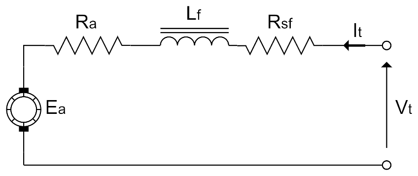
Figure 2: Series Excited DC Motor Equivalent Circuit
In a series DC motor, as suggested by the name, the field winding is connected in series with the armature. Unlike a separately excited field winding, which tends to have lower current and a high number of turns, the series field winding has a low number of turns, low resistance and is capable of taking the full armature current. The equivalent circuit diagram can be seen in Figure 5.
The armature circuit equation for a series motor may be written as
\[V_{t} = I_{t}R_{s} + E_{a}\]
where total series resistance Rs is the sum of armature resistance Ra and series field winding resistances Rsf:
\[R_{s} = R_{a} + R_{\text{sf}}\]
Since the armature and field winding are in series:
\[I_{t} = I_{a} = I_{f}\]
In a series motor, the field winding is often assumed to be non-saturating. Therefore following linear equation can be used. Where c is a constant:
\[\phi = cI_{t}\]
Substituting (11) into (1), (2) and (10) we can rearrange the equation to get the torque speed relationship for a series motor.
\[\omega_{m} = \frac{V_{t}}{\sqrt{\text{kc}}} \bullet \frac{1}{\sqrt{\tau_{\text{dev}}}} - \frac{R_{s}}{\text{kc}}\]
Comparing (7) and (12), the torque-speed characteristics of separately excited and series excited DC motors are quite different. For both machines, speed is proportional to terminal voltage. However the torque relationships are quite different. The main reason for the difference is that flux is a function of armature current.
The primary method of speed control for series DC motors is to control the terminal voltage. Controlling the terminal voltage directly impact both the field and armature windings.
Again, it is important to consider the limitations imposed by the torque-speed equation. Considering (12) one can see that as the torque falls to zero (no load is applied), the speed will theoretically reach infinity. Caution must be exercised to make sure that a load is applied before the motor is switched on.
3 Pre-lab
The Pre-lab is to be completed and handed-in at the beginning of your schedule lab session. You will not be allowed to participate in the Laboratory Experiments until your Pre-lab has been completed.
3.1 Pre-lab Reading
Familiarize yourself with the lab procedures and requirements by reading through the lab manual.
Familiarize yourself with the Safety Rules as well as the Equipment and Software used in the third Laboratory by viewing the information on the laboratory webpage below:
https://sites.google.com/a/ualberta.ca/ece332—electrical-machines
Note the equipment datasheets can be located at the bottom each page.
To access the webpage, you need to be logged-in with your CCID.
Re-watch the ‘General Lab Safety’ video available on eClass.
Review DC motor theory.
Have at least, the ‘ECE332 -Lab 1 – Signoff’ sheet printed off before coming to the lab.
3.2 Pre-lab Questions
The information for questions 1-7 can be found either in the Lab 1 manual or on the webpage and datasheets mentioned above. Answer the questions on a separate piece of paper to be handed-in at the beginning of your schedule lab session (Show all of your work). Make sure you put your clearly put your name, student ID number, CCID and your lab section at the top of the page.
What are the 4 test circuits that are in this lab?
What are the ratings for following parameters of the DC motor (Model 8211-00) used in the lab.
Motor Output Power
Generator Output Power
Full Load Speed
Full Load Motor Current
What Device is used to mechanically load the DC motor in the lab? Explain briefly how this device is constructed and operated? How is the motor coupled to this mechanical load?
For a separately excited DC machine:
Explain why you should power up the field circuit before the armature circuit?
Explain the effect on motor speed if you decrease the field current?
What theoretically happens to the series DC motor if you operate it with no-load?
Explain why DC motors can experience large starting currents when an instantaneous armature voltage is applied? Name and describe a method to limiting the starting current?
Compare the following attributes of a series field winding and shunt field winding in a DC Motor:
Wire Diameter
Current carrying capability
Number of turns
DC Resistance of winding
4 Lab Procedure
Login to the computer at your station. Use your CCID and password.
Connect and power the Data Acquisition and Control Interface (DACI) and launch the LVDAC-EMS software.
Make sure you use 120V, 60Hz for your system voltage and frequency
Make sure the Work in standalone mode is unchecked.
4.1 Circuit 1 - DC Resistance Tests
In this test you will apply a DC voltage to the armature, shunt field and series field windings, one at a time, while measuring the voltage across and the current through to determine each windings DC resistance.
4.1.1 Circuit Setup
Connect the circuit shown in Figure 2.
Use the Variable DC Supply
Use I1 and E1 to measure the DC Current and Voltage in the armature.
The Series and Shunt Field are shown because once you complete the measurement of the armature resistance you will first replace the armature with the series field then the shunt field to obtain their resistance values as well.
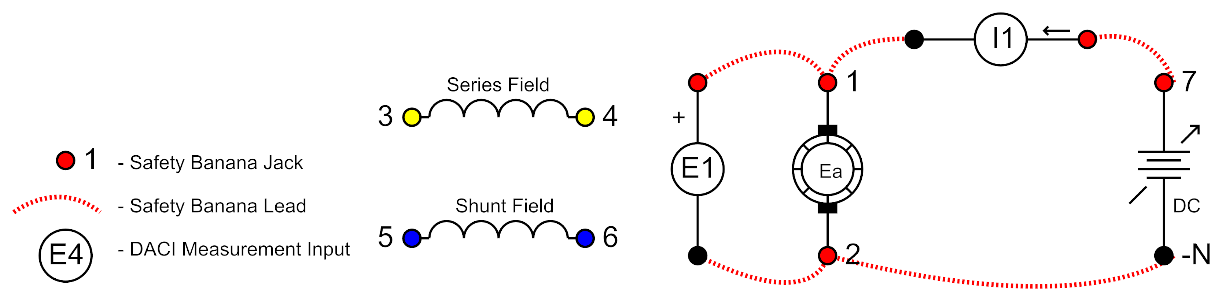
Figure 3: Circuit 1 (DC Resistance Measurement Circuit)
4.1.2 Instrument Setup
- Setup the Metering Instrument as follows in Table 1:
| Meter | Description | Type | Input/ Function | Mode |
|---|---|---|---|---|
| M1 | DC Voltage | Voltage | E1 | DC |
| M2 | DC Current | Current | I1 | DC |
| M3 | DC Resistance | Impedance | RDC (E1, I1) | R |
4.1.3 Results
To measure the armature winding resistance follow the steps (i-viii) in the DC Resistance Measurement Procedure.
Replace the armature winding in Figure 2 with the series field winding and repeat the DC Resistance Measurement Procedure.
Again, replace the item under test in Figure 2 with the shunt field winding and repeat the DC Resistance Measurement Procedure.
4.1.3.1 DC Resistance Measurement Procedure.
When you think your circuit and instrumentation is setup correctly get an instructor or TA to verify it before you apply power.
Make sure the variable voltage power supply variac is at 0%
Apply power by using the main power switch, L1, L2 and L3 should light up to indicate power.
Make sure that you have hit continuous refresh on the meter display and that it’s refreshing.
While adjusting the variac always keep an eye on the value of I1. You should never allow the value to increase excessively above the rated value of the device under test; (3 amps for the armature and series field windings and 0.4 amp for the shunt field winding). For the armature test, if the machine begins to rotate due to residual magnetism in the field. Make sure you quickly return the variac to zero and instead of using the rated current as your test point use a lower armature current where the machine is not rotating.
Adjust the variac until you get to an appropriate winding current as mentioned above.
Record the voltage, current and resistance from the meter into the appropriate table in the results section.
Adjust the power supply variac back to 0% and turn off the main power supply.
Once you complete all 3 tests for the winding resistances get an instructor or TA to sign-off on your results sheet.
Return the main power supply variac to 0% and turn off the main power supply. Disconnect your circuit.
4.2 Circuit 2 - No-load Separately Excited Tests
For this circuit you will connect a separately excited DC motor and run it with no mechanical load connected. You will do 2 separate tests: the first, you will maintain a constant shunt field current and change the armature voltage supply to see how speed is affected. In the second, you will maintain a constant armature voltage and adjust the shunt field current to again see how this affects speed.
4.2.1 Circuit Setup
Connect the circuit shown:
Connect the fixed DC voltage supply to the shunt field circuit
Be sure to include the field rheostat on the DC Motor panel in series with the shunt field winding.
Include I2 and E2 to measure the current and voltage of the shunt field winding.
Connect the variable DC voltage supply the armature.
- Include I1 and E1 to measure the current and voltage of the armature winding.
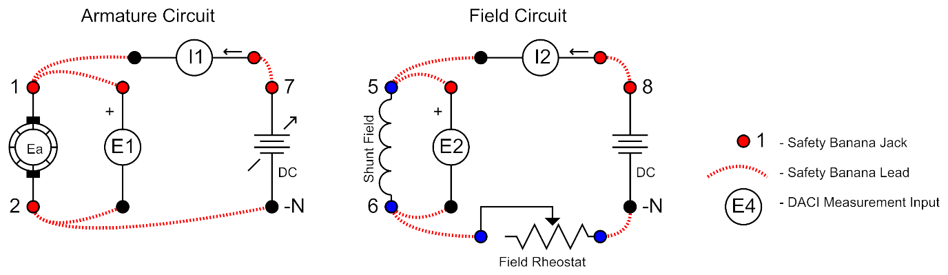
Figure 4: Circuit 2 (Shunt Tests)
4.2.2 Instrument Setup
Setup the Metering Instrument as shown in Table 2:
M1, M2 and M3 are for monitoring the armature winding.
M7, M8 and M9 are for monitoring the field winding.
It is recommend to create appropriate labels for each meter to avoid confusion.
| Meter | Description | Type | Input/ Function | Mode |
|---|---|---|---|---|
| M1 | Armature Voltage | Voltage | E1 | DC |
| M2 | Armature Current | Current | I1 | DC |
| M3 | Armature Power | Power | PQS1(E1,I1) | P |
| M7 | Shunt Field Voltage | Voltage | E2 | DC |
| M8 | Shunt Field Current | Current | I2 | DC |
| M9 | Shunt Power | Power | PQS2(E2,I2) | P |
4.2.3 Results (Constant Current)
When you think your circuit and instrumentation is setup correctly get an instructor or TA to verify it before you apply power.
Make sure the variac is at 0%
Apply power by using the main power switch, L1, L2 and L3 should light up to indicate power.
Make sure that you have hit continuous refresh on the meter display and that it’s refreshing.
Adjust the field rheostat on the DC motor panel until you get a shunt field current of 350 mA. Try and keep this value constant at 350mA throughout this test.
Change the knob on the main power supply to 7-N to read the variable DC supply voltage.
Increase the voltage across the armature slightly by increasing the main variac until the motor starts to rotate, check that the rotation direction is the same as that indicated on the Electrodynamometer panel. If the direction is wrong, turn off power and double check your circuit connections.
Increase the voltage across the armature to 120V and record the values from the metering instrument either by using the table provided in the results section or using the Data Table. You may need to wait a a few seconds or so until your values stabilize due to the temperature changes happening in the motor.
Measure the speed of the shaft by using the handheld tachometer and record this in the table as well.
Repeat these measurements for 100 V to 20 V with decrements of 20 V.
Once complete return the power supply variac back to 0%, but leave the circuit connected.
4.2.4 Results (Constant Voltage)
Adjust the Rheostat on the DC Motor panel so you get a maximum field current.
Increase the voltage across the armature to 80V and you may need to wait a minute or so for your values to stabilize due to the temperature changes happening in the motor. Try and keep this value constant at 80 V throughout this test. Once the meters are somewhat stable, record the values from the metering instrument either by using the table provided in the results section or using the Data Table.
Measure the speed of the shaft by using the handheld tachometer and record this in the table as well.
Repeat these measurements for a shunt field current of 400mA down to the minimum setting at decrements of 50mA, include the minimum settings.
Once Complete, turn the power supply variac to 0% and turn off the supply.
Get an instructor or TA to view your results and sign off on your results sheet. Leave the circuit connected.
4.3 Circuit 3 - Separately Excited Load Test
For this circuit you will add an adjustable mechanical load to DC motor. You will operate the machine at a fixed armature voltage and field current and see how the DC motor responds to different load levels.
4.3.1 Circuit Setup
Connect the circuit shown:
- Add a fixed single-phase (phase to neutral) power supply to the electrodynamometer load to the already connected circuit from the previous section as shown in Figure 4.
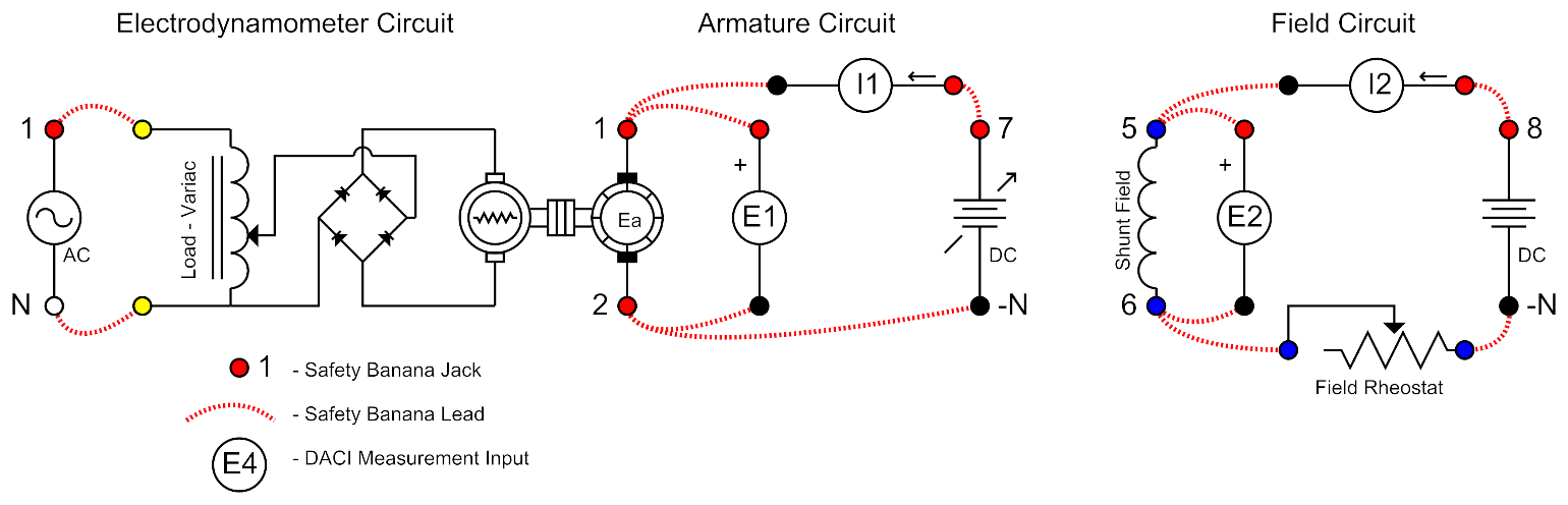
Figure 5: Circuit 3 (Separately Excited Load Test)
- The Electrodynamometer is a controllable mechanical load that you will use to load the DC motor. You control it by changing the load-variac setting, where at 0% it is at no-load and increases the load the higher you go. However the increase is non-linear, so when operating you will get almost no load change initially and once you hit a certain level the torque will increase quickly. Caution must be taken due to quick changes in load can cause the load to oscillate. To prevent oscillations it is best to make changes slowly.
4.3.2 Instrument Setup
- Leave the Metering Instrument Setup the same from the previous section shown in Table 2.
4.3.3 Results
When you think your circuit and instrumentation is setup correctly get an instructor or TA to verify it before you apply power.
Make sure the variac is at 0%
Apply power by using the main power switch, L1, L2 and L3 should light up to indicate power.
Make sure that you have hit continuous refresh on the meter display and that it’s refreshing.
Adjust the field rheostat on the DC motor panel until you get a shunt field current of 350 mA. Try and keep this value constant at 350mA throughout this test.
Increase the voltage across the armature by adjusting the power supply variac to 80V. Try and keep this value constant at 80V throughout this test.
Increase the load-variac on the electrodynamometer to increase the torque on the DC motor. Watch the armature current carefully. Do not excessively exceed the current rating of the armature winding (3 Amps). Increase the load until you get an armature current of approximately 3 Amps.
Record the values from the Metering Instrument either by using the Table provided in the results section or using the Data Table. You may need to wait a minute or so for your values to stabilize due to the temperature changes happening in the motor. Also don’t take measurements while the load is oscillating.
Measure the speed of the shaft by using the handheld tachometer and record this in the table as well.
Measure the torque by recording the value currently displayed on the Newton-meter scale on the Electrodynamometer.
Repeat these measurements by adjusting the load-variac for armature currents of 2.5 Amps to no-load decrementing the armature current by 0.5 Amps for each step. Include the minimum load setting. Remember to maintain 80V and 350mA. Record the Results in the appropriate table in the result section.
Once complete return electrodynamometer variac to 0%, the armature power supply variac back to 0% and turn off the main supply.
Get an instructor or TA to view your results and sign off on your results sheet. Leave the circuit connected.
4.4 Circuit 4 - Series Connected Field Load Test
4.4.1 Circuit Setup
Reconfigure the circuit as shown in Figure 6:
Leave the Electrodynamometer connected as is.
Connect the DC motor armature in series with the series field. Make sure the terminal 1 of the armature is connected to terminal 4 of the series field.
Use the variable DC supply to power the DC motor while using I1 and E1 to monitor the motor current and voltage.
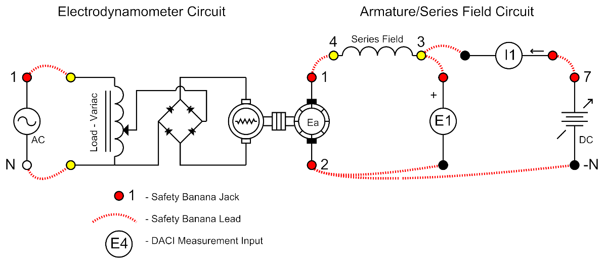
Figure 6: Circuit 4 (Series Connected Load Test)
4.4.2 Instrument Setup
- Setup the Metering Instrument as shown in Table 3:
| Meter | Description | Type | Input/ Function | Mode |
|---|---|---|---|---|
| M1 | Terminal Voltage | Voltage | E1 | DC |
| M2 | Terminal Current | Current | I1 | DC |
| M3 | Power | Power | PQS1 (E1, I1) | P |
4.4.3 Results
When you think your circuit and instrumentation is setup correctly get an instructor or TA to verify it before you apply power.
Make sure the main power supply variac is at 0%
Apply power by using the main power switch, L1, L2 and L3 should light up to indicate power.
Make sure that you have hit continuous refresh on the meter display and that it’s refreshing.
Adjust the load-variac on the Electrodynamometer panel to 30% to add some load for the series excited DC motor.
Increase the voltage across the armature by adjusting the power supply variac to 80V. Try and keep this value constant at 80V throughout this test. However watch the armature current, don’t excessively exceed the rated motor current (3 Amps). If the current exceeds 3 Amps prior to you obtaining 80V then turn down the load-variac.
Increase the load-variac until the motor current reaches 3 amps. It is very important to make all adjustments to the input voltage and load slowly. If you adjust things to quickly the load will oscillate.
Once you have the motor operating at 80 V and 3 A record the meter values in the table in the results section. Record the values from the metering instrument either by using the Table provided in the results section or using the Data Table. You may need to wait a minute or so for your values to stabilize due to the temperature changes happening in the motor. Also don’t take measurements while the load is oscillating.
Measure the speed of the shaft by using the handheld tachometer and record this in the table as well.
Measure the torque by recording the value currently displayed on the Newton-meter scale on the Electrodynamometer.
Repeat these measurements by adjusting the load-variac for armature currents of 2.5A, 2.0A and 1.5A. Record all of the results in the appropriate table.
Once complete first turn down the main power supply variac slowly and once the DC motor stops you can also turn down the electrodynamometer load-variac to 0%, then turn the main power supply off.
Get an instructor or TA to view your results and sign off on your results sheet. Leave the circuit connected.
4.5 Clean Up
Verify your results with an instructor or TA to show that you have completed everything.
Cleanup your station, everything should be returned to where you got it from.
Once everything is completed and tidy get a signature on your Results page before you leave.
5 Postlab
5.1 Results Spreadsheet
Once you have all the required measurements recorded download the spreadsheet called “ECE332 – Lab 3 – Results.xlsx” on the ECE332 eClass webpage under Lab 3. Copy your results into the provided spreadsheet. It will automatically calculate all the required information and plot the required graphs. Print a copy of the spreadsheet tabs Results and Graph to hand in with your report.
5.2 Sample Calculations
The following sample calculations must be handed in with your results. Use the methods that are discussed in the lab manual. (Show all your work):\
5.2.1 Separately Excited
Using the no-load test data, calculate the value of kφ when Vt = 100V and If = 0.350A
Using the separately excited load data, calculate Ea, Pdev, Pout, and η for the case where Ia = 3.0A.
A speed of 1400rpm is required to be obtained in the separately excited DC motor using field–weakening (reducing If), while the armature voltage and current are held constant. Determine the τdev available at the speed of 1400rpm for the case of Ia = 3.0A.
5.2.2 Series Excited
Using the series motor experiment data, Calculate Ea, Pout, Pdev, τdev, η and the constant kc for the case where Ia = 2.0 A.
Assuming the series DC motor used in the lab is mechanically coupled to a fan load for the case of Ia = 3.0A, the speed is required to reduce to 600rpm by inserting an external resistance Rext in series with Rs. Vt is constant while changing Rsf. The torque required by a fan is proportional to the square of the speed. Neglect armature reaction and rotational losses, i.e. you can assume c is a constant in φ = cIa and τdev equals load torque. Determine the values of Rext and Ia required for the new speed.
5.3 Questions
Answer the following questions to hand in with your lab report.
5.3.1 Separately Excited
Is the relationship between no-load speed and terminal voltage linear (at constant field)? Explain why.
Is the relationship between no-load speed and field current (at constant terminal voltage) linear? Explain why.
Is the calculated torque developed equal to the measured torque? If not, suggest why.
The measured torque-speed curve may not be strictly linear, particularly at high torque. Suggest a possible reason for this phenomenon.
Explain why a separately excited motor may be suitable for a conveyor belt drive.
5.3.2 Series Excited
Describe the flux–current relationship.
Describe the two major components of losses in the system and their impacts on the efficiency plot.
How can the direction of rotation be reversed in a series DC motor?
Explain why a series motor may be suitable for a railway traction drive.