Lab 3: Transmission Lines

ECE330 - Introduction to Power Engineering

---

1 Introduction

In this lab ac transmission lines will be explored by constructing equivalent circuit models using simple passive components. These circuit models will be used to demonstrate various characteristics of typical high-voltage ac transmission lines that are used to transfer large amounts of electrical power throughout the world. The four circuits to be completed in the laboratory are as follows:

• Circuit 1: Voltage Regulation
• Circuit 2: Power-Voltage
• Circuit 3: Voltage Compensation
• Circuit 4: Effect of Length

1.1 Pre-lab

• Familiarize yourself with the lab procedures and requirements by reading through the lab manual.

• Familiarize yourself with the Safety Rules as well as the Equipment and Software used in the third Laboratory by viewing the information on the laboratory webpage below:

  https://sites.google.com/ualberta.ca/ece330-introtopowerengineering/home

  • Note the equipment datasheets can be located at the bottom each page.

  • To access the webpage, you need to be logged-in with your CCID.

  • If you cannot access the webpage contact: terheide@ualberta.ca

• Re-watch the General Lab Safety Video .

• Review Transmission Line theory.

• Have at least, the ECE330 - Lab 3 - Sign-off sheet printed off before coming to the lab.

• Review the ECE330 - Lab 3 - Results Sheet that is used to collect your results and make plots that are to be handed in for your post-lab.

1.1.1 Pre-lab Questions

The information for questions 1-7 can be found either in the Lab 3 manual or on the webpage and datasheets mentioned above. Answer the questions on a separate piece of paper to be handed-in at the beginning of your schedule lab session (Show all of your work). Make sure you clearly put your name, student ID number, CCID and your lab section at the top of the page.

1. Explain why are transmission lines are used at high voltages.

2. Explain the difference between a distributed-parameter and lumped-parameter equivalent circuit model.

3.Explain why it is important during the Voltage Regulation experiment to not increase the capacitive loading on the transmission line model by not allowing the reactance to go below 300Ω.

4.Explain what the characteristic impedance (Z 0) and natural load (P0) of a high-voltage ac transmission line are. Give the equations used to calculate the values of these parameters assuming that the line is lossless.

5.Explain how switch shunt compensation (SSC) is implemented on a transmission line while also discussing what it’s purpose is.

6. What are the 3 main undesirable effects that length have on a transmission line?

7.For the Effect of Length experiment 2 segments of lumped-parameter equivalent circuits are used to double the length of the transmission line, explain why the capacitor C2 is set to 600Ω while capacitors C1 and C3 are set to 1200Ω.

1.2 Equipment Required

List of Equipment used for this Laboratory Experiment.

• Power Supply – Model 8525-20
• Data Acquisition and Control Interface (DACI) – Model 9063
• Three-phase Transmission Line – Model 8329-00
• Resistance Load – Model 8311-00
• Inductive Load – Model 8321-00
• Capacitive Load – Model 8331-00
• Safety banana Leads – 3 Colors, 3 Lengths
• Computer running LVDAC-EMS software
• Accessories – (USB cable, Barrel Power Cable)

1.3 Background

Figure 1. AC transmission lines at sunset

The main purpose of a transmission line in a power system network is to efficiently transfer electrical power from one area to another, typically from a power generating station (the sender end of transmission lines) to the distribution network (the receiver end of transmission lines), which then supplies electrical power to consumers.

Electrical power is produced in different types of generating stations which are typically located near the source of power (ie. coal mine, hydroelectric dam, windy or sunny location etc…) and then transferred by transmission lines to where it can be used, typically to a city’s distribution system. The electrical power from the generating station is converted to a very high voltage (generally from about 150kV to about 765kV) by using a step-up transformer for use on the sender end of the transmission line and then converted again to a lower voltage at the receiver end using a step-down transformer. The very high voltage is used to decrease the current flowing through the transmission lines’ cables for the same amount of power. In turn, a lower current means there will be less I²R losses during the transmission making the transmission line more efficient. Transmission lines can have lengths on the orders of hundreds or thousands of kilometers.

Typical AC transmission lines consist of three line wires, one for each phase, with no neutral wire. Most transmission lines are aerial meaning that they are supported on large towers rather than underground. This is due to aerial lines being much cheaper even though some might think they aren’t aesthetically pleasing. The conductors used are usually made up of aluminum alloy reinforced with steel as this is seen as the best compromise between cost, weight, strength, and conductivity. The metal conductors typically have no insulation covering them as the conductors are kept physically separated on the towers.

1.3.1 Transmission Line Models

As we can’t physically do tests on real transmission lines in the lab for various obvious reasons (the distances required, the large voltages and the cost) we can simulate the transmission lines by using an equivalent circuit model.

1.3.1.1 Short Segment

If you visualize the transmission line conductors that travel over the ground for a long distance you can see it would have the following parameters:

• R - the conductors would have a resistance to them that is proportional to their length due to the resistive nature of the material used. The resistance is usually stated as ohms per kilometer (Ω/km).
• X_L - the conductors would have an inductance (ie. inductive reactance (X_L)) to them that is proportional to their length as even a single straight wire has some inductance. The inductive reactance is usually stated as ohms per kilometer (Ω/km).
• 2X_C - an electric field (ie. capacitance) is formed between the conductor and the ground that is also proportional to its length. The overall capacitance is typically lumped into two capacitors, one at each end of the transmission line model. As these two capacitors are used we divide the capacitance for the distance between them and this results in each capacitor having two times the reactance (ie. 2X_C). The capacitive reactance is usually stated as ohms per kilometer (Ω/km).

The figure below shows the equivalent electric pi circuit model for a short transmission line segment (eg. 1km)

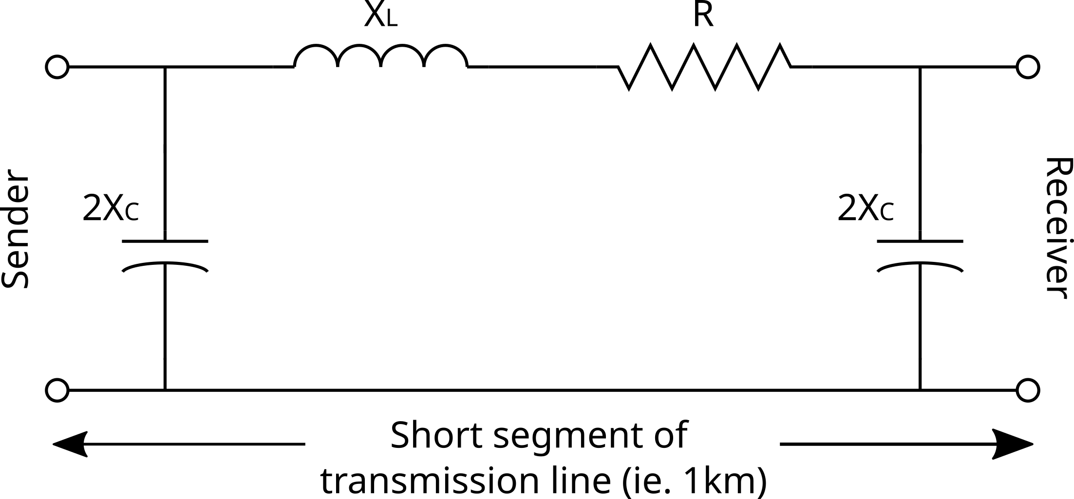
Figure 2. Equivalent circuit of a short segment of a distributed-parameter ac high-voltage transmission line

Note that the equivalent electric circuit in figure 2 only represents a short segment of one phase of an ac transmission line. For a complete three phase transmission line segment you can simply replicate the same circuit model three times, once for each phase, as shown in the figure below. Also note that the input and output connections for each phase are line-to-neutral.

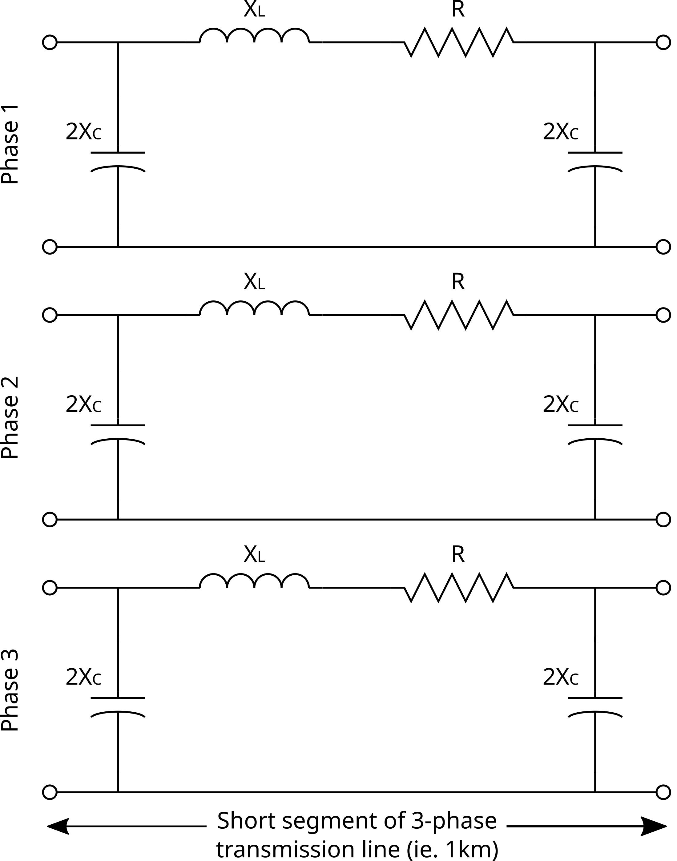
Figure 3. Three-phase equivalent circuit model

Below is an example of parameter values for the fundamental characteristics of a 315kV (line-to-line rms) high-voltage transmission line. These values depend on the physical dimensions and materials used in the construction of the transmission line. Note how the XL/R ratio is relatively large which is typical of high voltage transmission lines.

• Resistance | R = 0.022 Ω/km
• Inductive reactance | X_L = 0.36 Ω/km
• Capacitive reactance | X_C = 225 kΩ/km

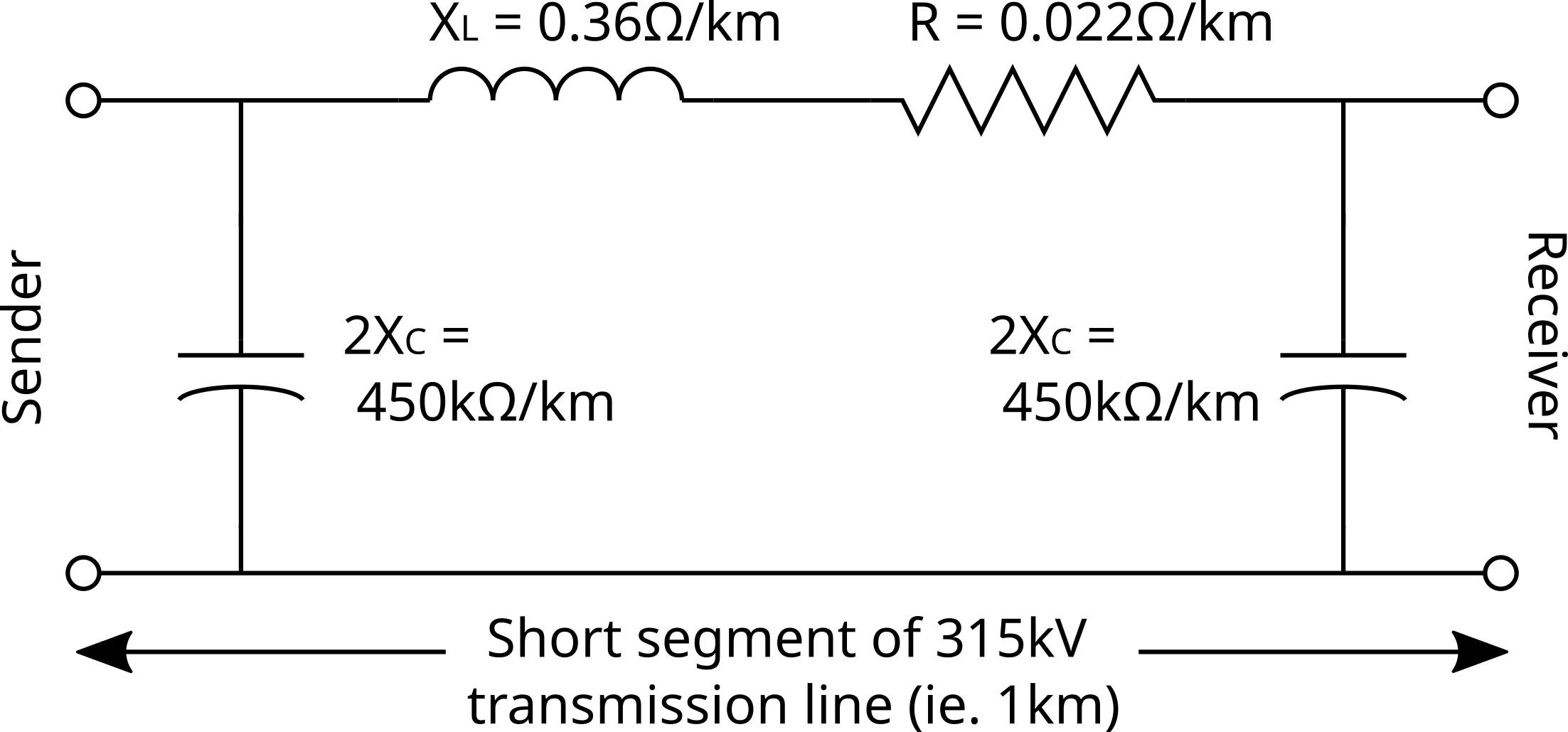
Figure 4. Short segment of an ac transmission line (1km)

1.3.1.2 Distributed-parameter

To obtain a model for a longer transmission line you can just string as many segments as required for the distance for a complete transmission line model as shown below. The resulting equivalent circuit is generally referred to as the distributed-parameter equivalent circuit. With small enough segments this type of equivalent circuit is considered an excellent representation of an ac transmission line and fully reproduces its electrical characteristics and behavior.

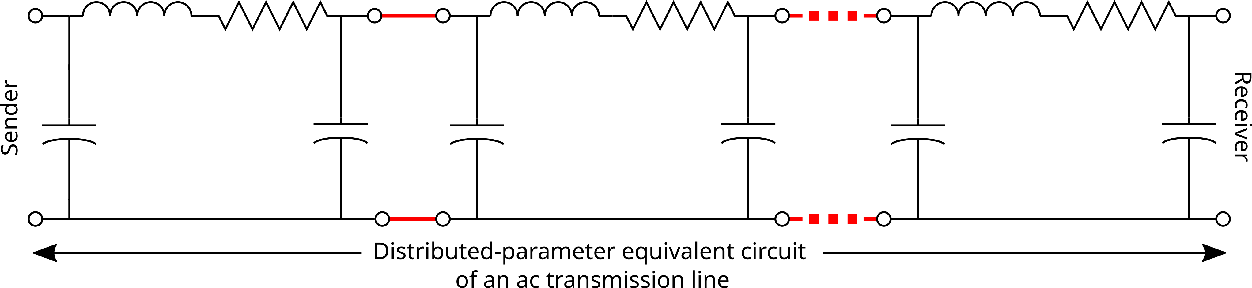
Figure 5. Distributed-parameter equivalent circuit

1.3.1.3 Lumped-parameter

To simplify calculation or in our case to limit the amount of components used to construct a transmission line model you can lump the parameters together. This can be done two ways. The first is known as the non-corrected PI equivalent circuit and does the following. Multiply the per kilometer segment resistance and inductive reactance and divide the capacitive reactance by the number of kilometers in the line to obtain the new model. The second is known as the corrected PI equivalent circuit and fixes a major problem of the first. As the line exceeds approximately 50 kilometers the voltage and the current at the sender and receiver ends of the non-corrected line no longer match and the characteristic parameters need to be tweaked so they do. The corrected PI equivalent circuit will provide very accurate results to about 625km. If the transmission line is longer than that you can simply break it up into smaller, shorter segments.

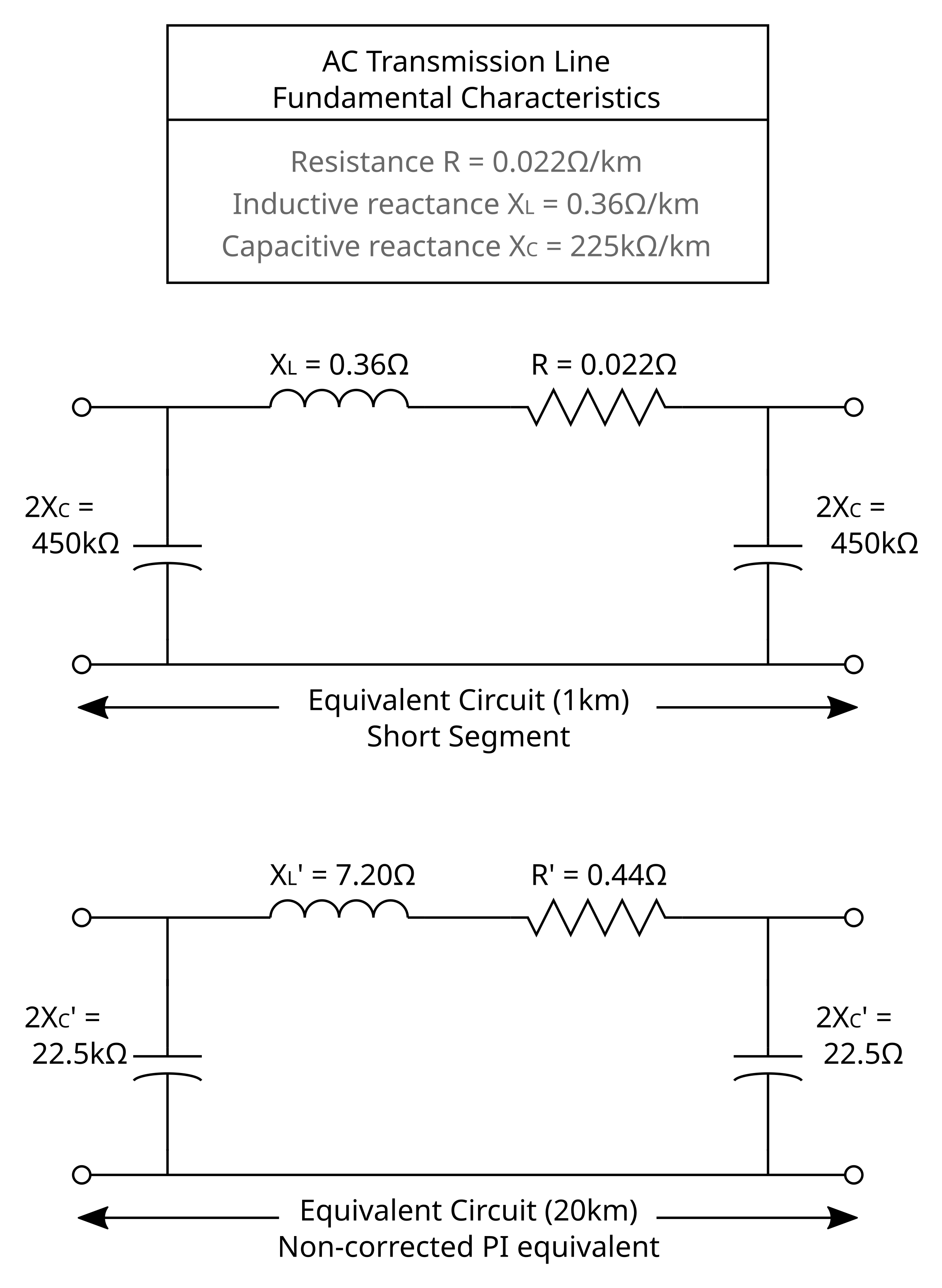
Figure 6. Example of a non-corrected pi equivalent circuit

1.3.1.4 Simplified Lumped-parameter

The simplified lumped-parameter equivalent circuit shown below does not fully reproduce the electrical characteristics and behavior of a high-voltage ac transmission line. It is simply a single inductor representing the entire inductance of the line. It is however a good first approximation and works best if used for only very short lines of about 20 kilometers or so. This circuit is useful in providing an introduction to the voltage regulation characteristics of ac transmission lines and will be used in the first circuit.

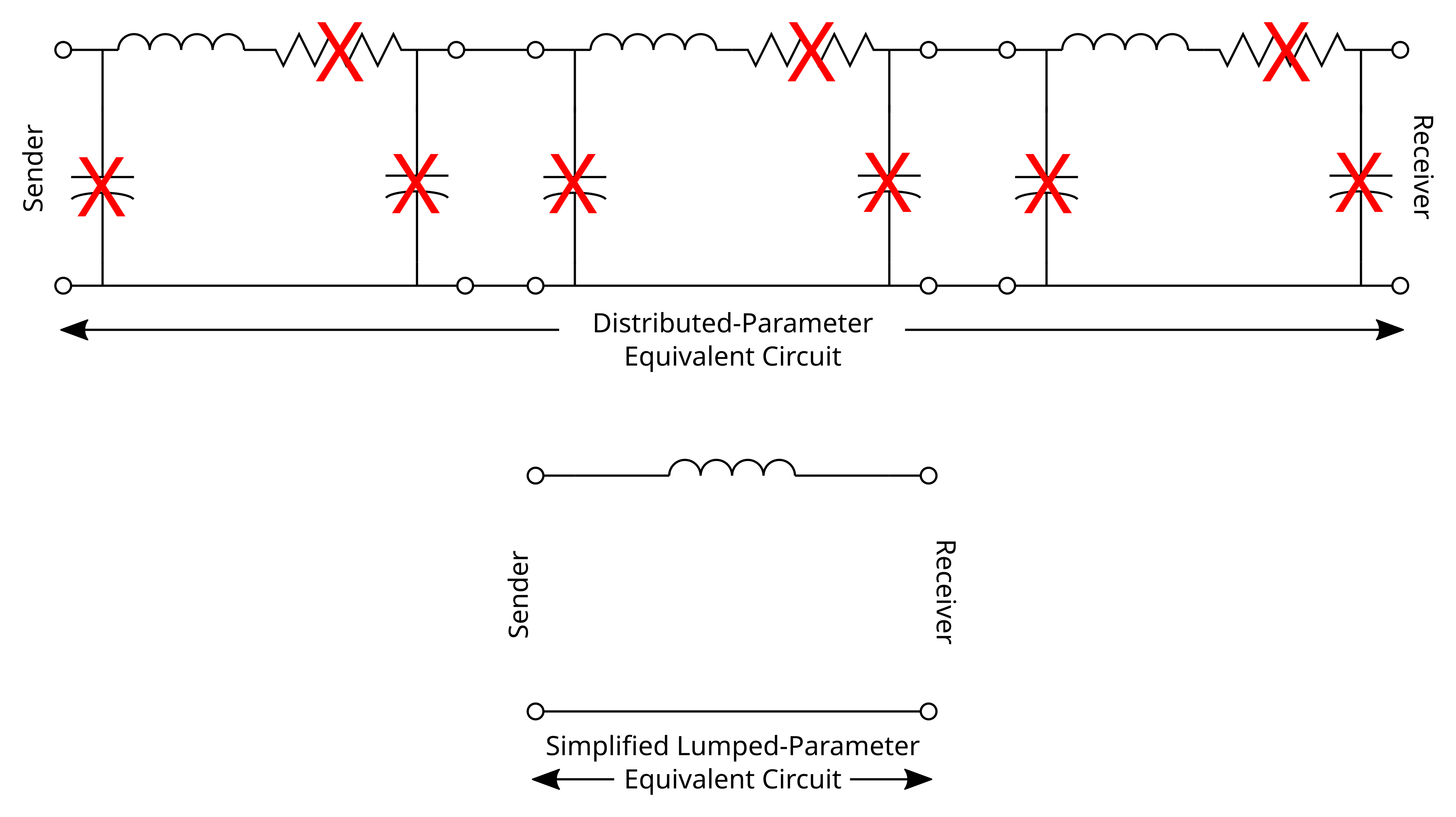
Figure 7. Simplified lumped-parameter equivalent circuit model

1.3.1.5 Recap - Transmission line models

1.3.2 Labvolt Module

The Three-Phase Transmission Line module has the same electrical properties as the simplified lumped-parameter equivalent circuit shown in figure 7 as there is simply a series inductor for each phase. The inductive reactance and therefore the length of the line can be selected with the knob on the front panel. There is also a switch on the front panel that disconnects the sender end (on the left, terminals labeled 1, 2, 3 and N) from the receiver end (on the right, terminals labeled 4, 5, 6 and N).

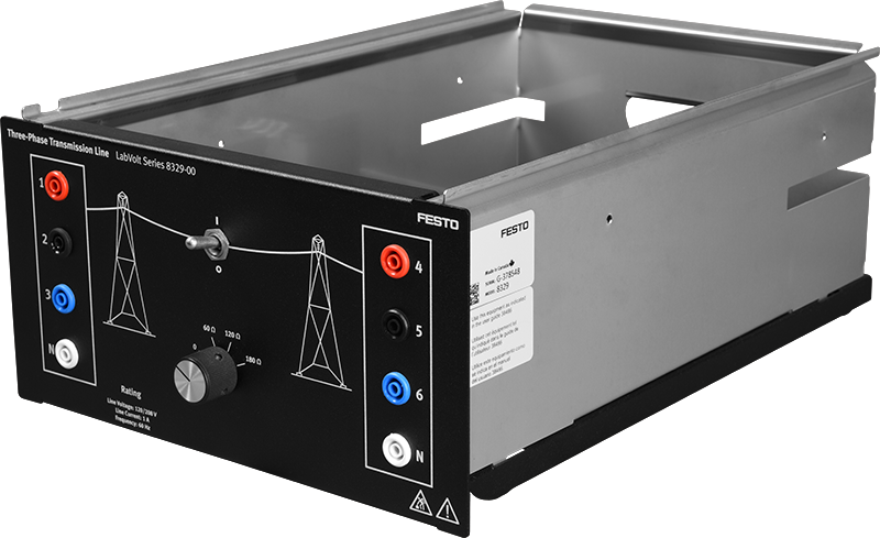
Figure 8. Labvolt Module 8329 - Three-phase Transmission Line

The three values that can be selected on the front are 60Ω, 120Ω and 180Ω. Remember that these values are for the inductive reactance of the transmission line. Note that the inductive reactance of a real aerial ac transmission lines operating at a frequency of 60Hz is generally between 0.30Ω/km to 0.50Ω/km. This is true no matter the operating voltage of the ac transmission line or power that is going through the ac transmission line. Therefore the approximate lengths of the lines that this model can convey are approximately 120km, 240km and 360km.

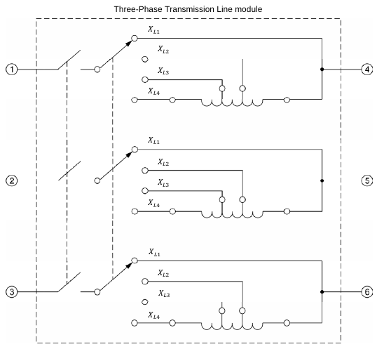
Figure 9. Labvolt Model 8329 - schematic

2 Experimental Procedure

2.1 Voltage Regulation

In this first test we want to determine how an ac transmission line’s receiver voltage varies while the sender end voltage is held constant and different loads are applied to the receiver end. The three different load types, resistive, inductive and capacitive, will be tested separately. Ideally, we would like for the sender and receiver voltages to stay at the same at all times. In practice this is difficult and therefore we specify how much the voltages differ using Voltage Regulation.

Voltage Regulation for a transmission line is defined as the following:

\[\text{Voltage Regulation (%)}= \frac{V_{NL} - V_{FL}}{V_{FL}} \times 100\%\] where

• V_NL is the no-load voltage at the receiver end of the ac transmission line, expressed in volts (V).
  
• V_FL is the full-load (or any-load) voltage at the receiver end of the ac transmission line, expressed in volts (V).

2.1.1 Circuit Setup

1. Connect the circuit shown in circuit 1.

   1. Connect the variable ac supply to power the sender end of the three-phase transmission line.

   2. First connect the Resistance Load to the receiver end of the Three-phase transmission line to use as the load impedance (Z1-Z3). During the lab we will change this impedance to both an Inductive and Capacitive Load.

   3. Connect E1 to measure the phase voltage on the sender end of the transmission line and E4 to measure phase voltage at the receiver end.

   4. Connect I4 to measure the red phase current at the output of the transmission line.

   5. Connect the Neutrals (N) of the power supply, transmission line and load.

Circuit 1. Voltage Regulation Circuit

2.1.2 Instrument Setup

2. On the Three-phase Transmission Line make sure the switch is in the on (I) position so the sender end is connected to the receiver end. Also adjust the knob on the three-phase transmission line to 120Ω to set the impedance/length of the transmission line.

3. Setup the Metering Instrument as follows:

Table 2. Metering Setup (Voltage Regulation)

Meter	Symbol	Description	Type	Input/ Function	Mode
M1	Z_Load	Load Impedance	Impedance	RXZ(E4,I4)	R/X
M2	Vs	Sender Phase Voltage	Voltage	E1	AC
M3	Vr	Receiver Phase Voltage	Voltage	E4	AC
M4	I	Phase Current	Current	I4	AC

2.1.3 Results

4. When you think your circuit and instrumentation is set up correctly, get an instructor or TA to verify it before you apply power.

5. After making sure the power supply variac is at 0% and that you have hit continuous refresh on the meter display and it is refreshing. Apply power by using the main power switch, L1, L2 and L3 should light up to indicate power.

6. With all 3 phases of the Resistive Load in the Open State indicated in the Load States table below, slowly increase the power supply variac to 100% while watching the meters to verify that everything is operating correctly. There should be nearly zero current and the sender and receiver voltage should be nearly identical.

7. Use the Data Table to record the 4 Meters you set up for all of the resistive Load States below, making sure to keep the three-phase load bank balanced (same resistance for each phase) for each reading.

8. Once you have captured readings for all of the Load States, export the Data Table to a .csv file making sure to indicate that this is the data for a resistive load. Save the file somewhere you will have access to after the lab.

9. Making sure to first turn off the power supply and return the variac back to zero. Change the Load used in the circuit from a Resistive Load to an Inductive Load. Make sure to maintain the voltmeter and ammeter connections.

10. After double checking your connections, turn the power supply on again and slowly increase the power supply variac to 100%, making sure that you are getting the correct readings.

11. Collect the same measurements you made for the resistive load for the inductive load. For Meter M1 you will need to change the Mode from R to X to get the correct reactance reading. Once all the measurements are complete export the Data Table to a .csv file making sure to indicate that this is the data for an inductive load. Save the file somewhere you will have access to after the lab.

12. Making sure to first turn off the power supply and return the variac back to zero. Change the Load used in the circuit from an Inductive Load to a Capacitive Load. Make sure to maintain the voltmeter and ammeter connections.

Caution!!!
As adding a large capacitor load to the transmission line can cause the receiver end voltage to increase beyond the ratings of the capacitors, it is important that you do not decrease the reactance of the capacitor load below 300Ω. Therefore for the capacitor load only obtain readings of Open, 1200Ω, 600Ω, 400Ω and 300Ω.

13. Collect the same measurements you made for the resistive and inductive load for the capacitor noting the Caution above. For Meter M1 you can leave the Mode on X to get the correct reactance reading. Once all the measurements are complete export the Data Table to a .csv file making sure to indicate that this is the data for a capacitive load. Save the file somewhere you will have access to after the lab.

14. Get an instructor or TA to view your .csv files and sign off on your results sheet.

15. Return the variac to 0%, and turn-off the main power supply.

2.2 Power-Voltage

In this second test we want to determine how the receiver voltage is affected by resistance of the load and how that load affects the amount of power following through the ac transmission line. For this test we will vary the resistance from open to short with many resistance values in-between in order to collect enough data to construct a Power-voltage curve. Note that we will also modify the equivalent circuit model for this circuit to include the appropriate capacitors to the sender and receiver ends of the line to create a pi circuit model similar to figure 6.

2.2.0.1 Voltage Regulation

Note that the voltage regulation characteristics of a high-voltage ac transmission line for a resistive load is actually slightly different then what was measured in the first experiment. Like in the first experiment an actual ac transmission line’s receiver voltage will decrease when the lines current increases, however, due to the capacitance of the transmission line the receiver voltage will exceed the sender voltage when a light load or no load is connected to the receiver end as shown below in the figure.

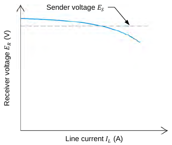
Figure 10. Plot showing the voltage regulation characteristic of an ac transmission line

From the figure above you can see that if you start loading an unloaded transmission line that the receiver voltage will decrease and at some point the receiver and sender voltages will equal each other. At this load point, the reactive power due to the parallel capacitance (Q_C) of the line equals the reactive power due to the series inductance (Q_L) of the line. At this particular operating point the line is said to be naturally balanced.

2.2.0.2 Calculate Z₀

The value of the load impedance required to make the receiver voltage equal to the sender voltage is known as the characteristic impedance Z₀. It can also be called the characteristic resistance in the case of a purely resistive load. The electrical characteristics of the ac transmission line determine its characteristic impedance and can be calculated using the equation below.

\[Z_0 = \sqrt{X_C \cdot X_L}\]

where

• X_L is the inductive reactance of the ac transmission line, expressed in Ω⁄km or Ω⁄mile.
  
• X_C is the capacitive reactance of the ac transmission line, expressed in Ω⁄km or Ω⁄mile.

For instance, we can calculate the characteristic impedance for the equivalent transmission line circuit model used in this section by using the components used. The inductive reactance that we are using is 120Ω. The total capacitive reactance is 600Ω after accounting for both the sender and receiver side capacitors and putting them in parallel.

\[ \notag Z_0 = \sqrt{120Ω \cdot 600Ω}\\ Z_0 = 268.3Ω \]

2.2.0.3 Calculate P_O

The active power delivered to a load at the receiver end of the ac transmission line when the load resistance equals the characteristic impedance Z₀ is referred to as the natural load P₀. The value of the natural load for a three-phase ac transmission line can be determined using the equation below.

\[P_0 = \frac{V_R^2}{Z_0} \cdot 3\]

where

• V_R is the phase voltage at the receiver end of the ac transmission line, expressed in V.
  
• Z₀ is the characteristic impedance of the ac transmission line, expressed in Ω.

For instance, we can calculate the natural load for our equivalent transmission line circuit model by using the characteristic impedance calculated above and assume that the receiver voltage equals the sender voltage that we apply at 120V. Note that we don’t need to multiple by 3 as we are only modeling a single phase system.

\[ \notag P_0 = \frac{120V^2}{268.3Ω}\\ P_0 = 53.67W \]

Note that two equations above are based on the assumption that the ac transmission line is lossless. In actual ac transmission lines, however, the resistance is not zero. Thus, the load impedance actually required to make the receiver voltage equal to the sender voltage is higher than the calculated characteristic impedance and as a consequence the active power actually supplied to the load is lower than the calculated natural load.

2.2.0.4 Power-Voltage Curve.

The figure below shows a typical complete voltage regulation characteristic for a high-voltage ac transmission line. This curve demonstrates how the transmission line behaves from no-load at the receiver end to short-circuit. Note that the y-axis shows the ratio of the receiver voltage relative to the sender voltage and the x-axis is the active power normalized relative to the natural load (P₀). This type of curve is also referred to as the power-voltage curve of the ac transmission line.

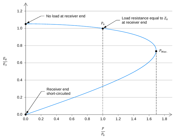
Figure 11. A typical power-voltage curve of an ac transmission line

2.2.1 Circuit Setup

As connecting the remaining circuits as three-phase circuits would require more equipment and becomes cumbersome to experiment on, we are only going to connect them as a single phase circuit or per phase circuit. The results would be similar for balanced circuits.

16. Connect the circuit in circuit 2 below by doing the following:

    1. Connect the variable AC supply to power the sender end of the transmission line. Use the E2 voltmeter to measure the sender end phase voltage and the I3 ammeter to measure the sender current.

    2. Connect capacitor C1 using one of the capacitors in the capacitive load bank to the sender end of the transmission line. Use the ammeter I2 to measure this capacitor’s current.

    3. Connect capacitor C2 using another one of the capacitors in the capacitive load bank to the receiver end of the transmission line. Use the ammeter I1 to measure this capacitor’s current.

    4. Add the resistor load bank to the receiver end of the transmission line by connecting the R1 bank in series with the R2 and R3 banks in parallel. Use the E4 voltmeter and I4 ammeter to measure the load’s current and voltage.

    5. Measure the voltage drop across the transmission line by connecting the voltmeter E3.

Circuit 2. Power Voltage Curve Circuit

2.2.2 Instrument Setup

17. On the Three-phase Transmission Line make sure the switch is in the on (I) position so the sender end is connected to the receiver end. Also adjust the knob on the three-phase transmission line to 120Ω to set the impedance/length of the transmission line.

18. The capacitors C1 and C2, which are part of the transmission line model, should both be set to 1200Ω.

19. Begin with all of the resistor load bank switches set to open.

20. Setup the Metering Instrument as follows:

Table 4. Metering Setup (Power Voltage Curve)

Meter	Symbol	Description	Type	Input/ Function	Mode
M1	R_Load	Load Resistance	Impedance	RXZ(E4,I4)	R
M2	Vs	Sender Phase Voltage	Voltage	E2	AC
M3	Vx	Voltage Across Transmission Line	Voltage	E3	AC
M4	Vr	Receiver Phase Voltage	Voltage	E4	AC
M7	I_Cs	Sender Capacitor Current	Current	I2	AC
M8	I_x	Transmission Line Current	Current	I3	AC
M9	I_Cr	Receiver Capacitor Current	Current	I1	AC
M10	I_Load	Load Current	Current	I4	AC
M13	P_Load	Load Power	Power	PQS4(E4,I4)	P
M14	Q_Cs	Sender Xc Reactive Power	Power	PQS2(E2,I2)	Q
M15	Q_x	Transmission Line Reactive Power	Power	PQS3(E3,I3)	Q
M16	Q_Cr	Receiver Xc Reactive Power	Power	PQS(E4,I1)	Q

2.2.3 Results

21. When you think your circuit and instrumentation is set up correctly, get an instructor or TA to verify it before you apply power.

22. After making sure the power supply variac is at 0% and that you have hit continuous refresh on the meter display and it is refreshing. Apply power by using the main power switch, L1, L2 and L3 should light up to indicate power. Slowly increase the power supply variac to 100% while watching the meters to verify that everything is operating correctly.

23. Use the Data Table to record the 12 Meters you set up for all of the resistive Load States below. 0 means the switch is off or open, 1 that the switch is closed and that that resistance is in the circuit. Short means the load bank is externally shorted using a safety banana plug, see the caution below.

Caution!!!
When shorting a load box to obtain the required resistance in the table below it is important that you turn off the ac power supply when doing so.

24. Once you have captured readings for all of the Load States, export the Data Table to a .csv file making sure to indicate that this is the data for the power voltage curve. Save the file somewhere you will have access to after the lab.

25. Get an instructor or TA to view your .csv file and sign off on your results sheet.

26. Return the variac to 0%, and turn-off the main power supply.

2.3 Voltage Compensation

In this third experiment we will be making the ac transmission line more useful by using switched shunt compensation to adjust the receiver voltage of the line, which varies due to the amount of loading, to more closely match the sender end’s voltage. In general, it is not desirable that the receiver voltage differs too much from the nominal value, as this is often a source of problems in any ac power network. As shown in the voltage regulation experiment we can adjust the voltage of the receiver end of the ac transmission line up or down by adding either a capacitive or inductive load, respectively.

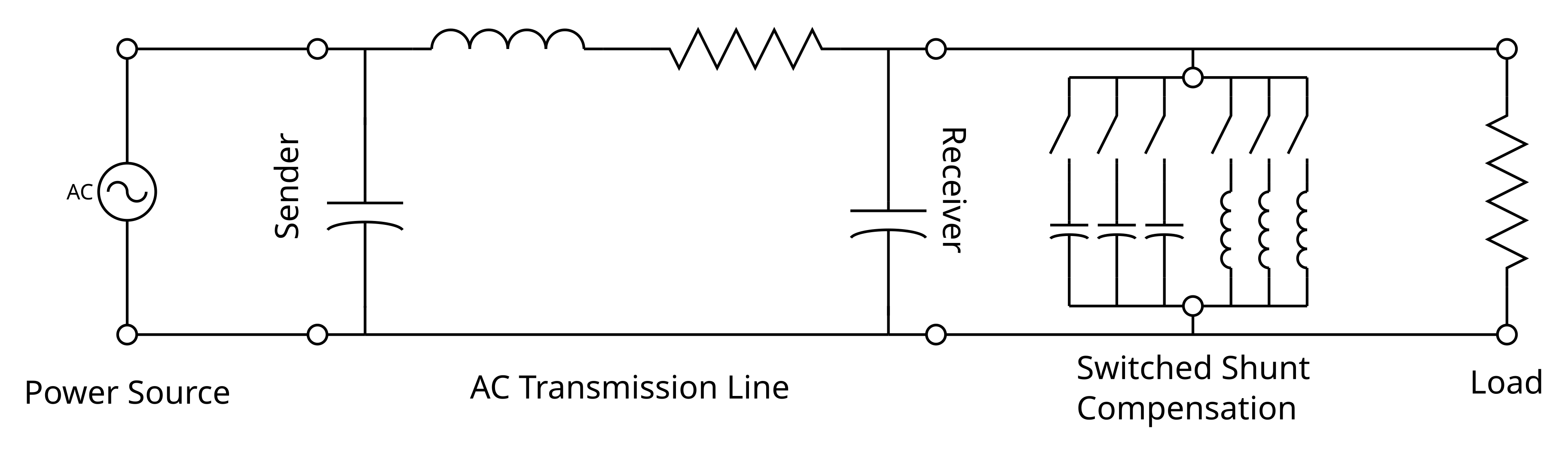
Figure 12. Circuit showing the switched shunt compensation circuit at the receiver end of an ac transmission line

During this experiment we are going to operate the ac transmission line model in a similar manner as the last experiment. However, now we are going to add the switched shunt compensation at the receiver end of the line and for each value of resistive load we are then going to compensate the receiver voltage by either increasing or decreasing it by adding the appropriate inductive or capacitive reactance at the load.

2.3.0.1 Power

The active power that is transmitted by a voltage compensated three-phase ac transmission line can be calculated from the formula below.

\[P_{Comp} = 3 \frac{V_S V_R}{X_L'}(\sin\delta)\]

where

• V_S - is the phase voltage at the sender end of the voltage-compensated ac transmission line, expressed in volts (V).
• V_R - is the phase voltage at the receiver end of the voltage-compensated ac transmission line, expressed in volts (V).
• X_L’ - is the inductive reactance in the corrected PI equivalent circuit of the ac transmission line, expressed in ohms (Ω).
• δ - is the phase shift between the receiver voltage and sender voltage , the receiver voltage being used as the reference voltage phasor [i.e., phase shift = phase angle phase angle, expressed in degrees (°)].

2.3.0.2 Maximum Power

The maximum amount of active power that a three-phase ac transmission line that has been voltage compensated can be calculated from the formula below.

\[P_{MAX} = 3 \frac{V_S V_R}{X_L'}\]

where

• V_S - is the phase voltage at the sender end of the voltage-compensated ac transmission line, expressed in volts (V).
• V_R - is the phase voltage at the receiver end of the voltage-compensated ac transmission line, expressed in volts (V).
• X_L’ - is the inductive reactance in the corrected PI equivalent circuit of the ac transmission line, expressed in ohms (Ω).

2.3.1 Circuit Setup

27. Modify the circuit from circuit 2 to obtain the circuit in circuit 3 below by doing the following:

    1. Remove the ammeters I1 and I2 from the circuit by replacing them and their connections with a single safety banana lead.

    2. Remove the voltmeter E3 from measuring the voltage across the transmission line.

    3. Add the shunt compensation circuit by first removing the load and inserting the remaining capacitor in the capacitance bank and the three inductor banks in series as shown below. Then, reconnect the load through the I4 ammeter to the shunt compensation circuit.

Circuit 3. Voltage Compensation Circuit

2.3.2 Instrument Setup

28. On the Three-phase Transmission Line make sure the switch is in the on (I) position so the sender end is connected to the receiver end. Also adjust the knob on the three-phase transmission line to 120Ω to set the impedance/length of the transmission line.

29. The capacitors C1 and C2, which are part of the transmission line model, should both be set to 1200Ω. The capacitor C3 is part of the switched shunt compensating (SSC) circuit and should begin in the open (not in the circuit) state.

30. The inductions L1, L2 and L3 are also part of the switched shunt compensating (SSC) circuit and should also begin in the open (not in the circuit) state.

31. Begin with all of the resistor load bank switches set to open.

32. Setup the Metering Instrument as follows:

Table 6. Metering Setup (Voltage Compensation)

Meter	Symbol	Description	Type	Input/ Function	Mode
M1	R_Load	Load Resistance	Impedance	RXZ(E4,I4)	R
M2	Vs	Sender Phase Voltage	Voltage	E2	AC
M3	Vr	Receiver Phase Voltage	Voltage	E4	AC
M4	I_Load	Load Current	Current	I4	AC
M5	P_Load	Load Power	Power	PQS4(E4,I4)	P
M6	PS	Sender/Receiver Phase Shift	Phase Shift	PS(E2,E4)	-

2.3.3 Results

34. When you think your circuit and instrumentation is set up correctly, get an instructor or TA to verify it before you apply power.

35. After making sure the power supply variac is at 0% and that you have hit continuous refresh on the meter display and it is refreshing. Apply power by using the main power switch, L1, L2 and L3 should light up to indicate power. Slowly increase the power supply variac to 100% while watching the meters to verify that everything is operating correctly.

36. Note that at this operating point the receiver voltage is greater than the sender voltage. As this is undesirable we are going to use the switched shunt compensation (SSH) to correct the receiver voltage by adding inductance at the receiver end of the transmission line. To correct this voltage we need to add about 1200Ω to make the sender and receiver voltages approximately equal. To get this we need to make L1 and L2 equal to 300Ω and L3 equal to 600Ω. Go ahead and do this and see the result.

37. Use the Data Table to record the 6 Meters you set up for all of the resistive load states below. Note that for each load state that the switched shunt compensation value that should be used are given and are the available values that should make the receiver voltage approximately equal the sender voltage. Refer to table 4 used in the previous section if you need help determining how to configure each load state.

38. Once you have captured readings for all of the Load States, export the Data Table to a .csv file making sure to indicate that this is the data for the voltage compensation. Save the file somewhere you will have access to after the lab.

39. Get an instructor or TA to view your .csv file and sign off on your results sheet.

40. Return the variac to 0%, and turn-off the main power supply.

2.4 Effect of Length

In this last experiment we are going to effectively double the length of the ac transmission line by adding another transmission line segment to demonstrate the effect that length has on the line’s Power-Voltage curve. This setup also allows us to measure the voltage halfway across a compensated ac transmission line which allows the demonstration that the line has a non-constant voltage profile along it.

2.4.0.1 Z₀ and P₀

Note that the length of an ac transmission line has no effect on the fundamental characteristics (R, X_L and X_C) of the line. These parameters all have the units in ohms per kilometer and therefore aren’t affected. Consequently, the characteristic impedance (Z₀) is also independent of the line’s length. Furthermore, the natural load (P₀) is also unaffected by length since it only depends on the characteristic impedance (Z₀) and the receiver end voltage.

Also note that when using a lumped parameter equivalent circuit that the parameters need to be corrected for line lengths that exceed approximately 50km to obtain accurate results. Below is an example of 2 corrected PI equivalent circuits for an ac transmission line at two different lengths.

Figure 13. Example of Lumped-parameter Corrected PI Equivalent Circuits for 2 Different Lengths of ac Transmission Line

2.4.0.2 Power-Voltage Curve

The figure below shows the Power-Voltage curves of the 250km and 500km lines from above.

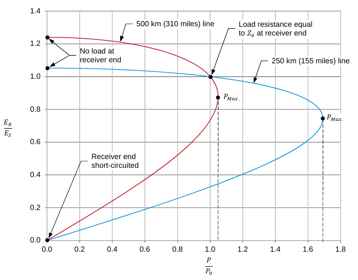
Figure 14. Example of how length affects the power-voltage curve of an ac transmission line

The following undesirable effects due to the ac transmission line length increasing can be observed when comparing the power-voltage curve of these two ac transmission lines.

1. Increasing the length makes the voltage at the receiver end increase significantly when the line is unloaded. This results in a more severe over-voltage condition when the load is lost for some reason and can cause damage to the line itself or the connected equipment.

2. Increasing the length makes the maximal active power (P_MAX) that the line can convey to the load decrease significantly. This is undesirable as you simply can not transfer as much power.

3. Increasing the length makes the change in the receiver voltage, when the load is changed, increase significantly. These increased fluctuation of the receiver voltage make the transmission line less stable and in turn can contribute in reducing the stability of the ac power network.

2.4.0.3 Voltage Profile

For an unloaded ac transmission line where the sender and receiver voltage are compensated the following voltage profile in the figure below will be apparent along the distance of the line. Note that the middle of the line will have the largest or maximal voltage.

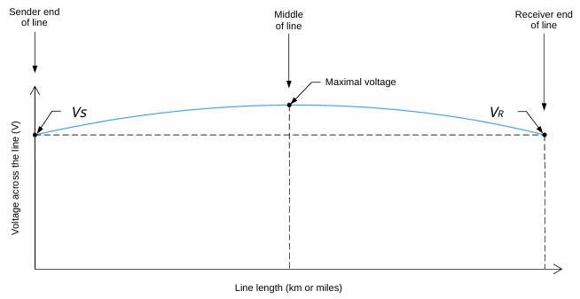
Figure 15. Example of the voltage profile over the length of an ac transmission line

The length of the ac transmission line will have an effect on the maximal voltage as shown in the figure below.

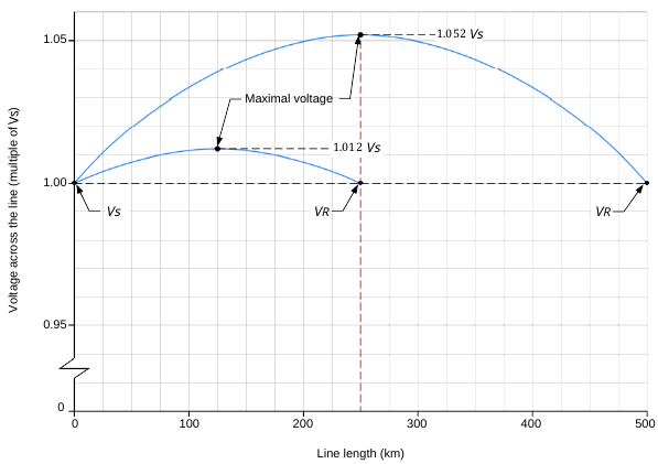
Figure 16. Example of the effect the length has on the voltage profile of an ac transmission line

2.4.1 Circuit Setup

41. Modify the circuit from circuit 3 to obtain the circuit in circuit 4 below by doing the following:

    1. Disconnect the capacitor C2 from the receiver end of the transmission line and the capacitor C3 in circuit 3. Then reconnect C2 at the sender end of the transmission line between the black phase and neutral. Use the voltmeter E3 to measure the voltage across this capacitor which will now be the center of this new transmission line that is twice as long as the previous one.

    2. Reconnect the capacitor C3 to the new receiver end of the transmission line by connecting it between the black phase and neutral.

    3. Remove the L3 inductor bank from the switched shunt compensation so that the compensation circuit only has 2 inductor banks in series instead of 3.

Circuit 4. Effect of Length Circuit

2.4.2 Instrument Setup

42. On the Three-phase Transmission Line make sure the switch is in the on (I) position so the sender end is connected to the receiver end. Also adjust the knob on the three-phase transmission line to 120Ω to set the impedance/length of the transmission line.

43. The capacitors C1, C2 and C3 which are all part of the new lengthened 2-segment transmission line model should be set to the following: C1 and C3 should be set to 1200Ω and the capacitor in the middle of the line C2 should be set to 600Ω.

44. The inductors L1 and L2 which form the new switched shunt compensating (SSC) circuit, should begin in the open (not in the circuit) state.

45. Begin with all of the resistor load bank switches set to open.

46. Setup the Metering Instrument as follows:

Table 8. Metering Setup (Effect on Length)

Meter	Symbols	Description	Type	Input/ Function	Mode
M1	R_Load	Load Resistance	Impedance	RXZ(E4,I4)	R
M2	Vs	Sender Phase Voltage	Voltage	E2	AC
M3	V_middle	Middle Phase Voltage	Voltage	E3	AC
M4	Vr	Receiver Phase Voltage	Voltage	E4	AC
M5	I_Load	Load Current	Current	I4	AC
M6	P_Load	Load Power	Power	PQS4(E4,I4)	P

2.4.3 Results (Power-Voltage)

47. When you think your circuit and instrumentation is set up correctly, get an instructor or TA to verify it before you apply power.

48. After making sure the power supply variac is at 0% and that you have hit continuous refresh on the meter display and it is refreshing. Apply power by using the main power switch, L1, L2 and L3 should light up to indicate power. Slowly increase the power supply variac to 100% while watching the meters to verify that everything is operating correctly.

49. Use the Data Table to record the 6 Meters you set up for all of the resistive Load States below (which is the same as the previous 2 circuits). 0 means the switch is off or open, 1 that the switch is closed and that that resistance is in the circuit. Short means the load bank is externally shorted using a safety banana plug.

Caution!!!
When shorting a load box to obtain the required resistance in the table below it is important that you turn off the ac power supply when doing so.

50. Once you have captured readings for all of the Load States, export the Data Table to a .csv file making sure to indicate that this is the data for the effect on length power voltage curve. Save the file somewhere you will have access to after the lab.

2.4.4 Result (Middle of Line)

51. Return the resistive load bank to its original No-load state and use the switched shunt compensation inductors to compensate the transmission line so the receiver voltage equals the sender voltage. What you will notice is that at the middle of the transmission line the voltage is larger than the nominal voltage at the sender and receiver end. This voltage could be potentially large enough to cause damage to the transmission line.

52. Use the Data Table to record the 6 Meters you set up for this test-point and then export the Data Table to a .csv file making sure to indicate that this is the data for the middle of the line. Save the file somewhere you will have access to after the lab.

53. Get an instructor or TA to view your .csv file and sign off on your results sheet.

54. Return the variac to 0%, and turn-off the main power supply.

2.5 Clean Up

1. Verify your results with an instructor or TA to show that you have completed everything.

2. Cleanup your station, everything should be returned to where you got it from.

3. Once everything is completed and tidy, get a signature on your Results page before you leave.

3 Post-lab

Lab Reports are due approximately 1 week after you attend your lab section, check eClass for the exact time. All reports need to be submitted to the appropriate link as a single pdf on eClass. You only have to hand-in one copy per group. Please have your pages in a single pdf file in the following order:

• Use a scanned/picture copy of the ECE330 - Lab 3 - Sign-off sheet as your cover sheet. Make sure your names, student ID’s, CCID’s and lab section are visible in the table at the top of the page. You need to obtain LI/TA signatures for completing each circuit during the Laboratory exercise.

• A pdf of the completed ‘Results’ worksheet from the ECE330 - Lab 3 - Results Sheet .

• The completed sample calculations (showing all of your work).

• The answers to the post lab questions.

3.1 Sample Calculations

The following sample calculations must be handed in with your results. Use the methods that are discussed in the lab manual. (Show all your work):

1. Calculate the voltage regulation for the Voltage Regulation experiment for 400Ω for all 3 load types, resistive, inductive and capacitive.

2. For the results for the Power-Voltage experiment calculate the total reactive power consumed by the ac transmission line when it is resistively loaded near the lines characteristic impedance (Z₀).

3. For the Voltage Compensation circuit calculate the active power when the line is resistively loaded by 500Ω using the following equation and compare it to the measured power. Note that the equation below is for a three-phase circuit and the experiment was only completed as a single phase circuit or as a per phase model.

\[P_{Comp} = 3 \frac{V_S V_R}{X_L'}(\sin\delta)\]

3.2 Questions

Answer the following questions to hand in with your lab report.

1. What happens to the receiver voltage of a simplified ac transmission line connected to a capacitive load as the line current increases? Explain why this happens.

2. What happens to the receiver voltage of a simplified ac transmission line connected to a resistive load as the line current increases? What happens if the simplified ac transmission line is connected to an inductive load instead?

3. What happens to the receiver voltage of a high-voltage ac transmission line connected to a resistive load as the line current increases? What happens if no load is connected to the receiver end of the high-voltage ac transmission line? Explain why this happens.

4. When is a lossless high-voltage ac transmission line naturally balanced?

5. Describe what the complete voltage regulation characteristic (Power-Voltage curve) of a high-voltage ac transmission line is. According to this characteristic, can any ac transmission line be operated beyond the natural load (provided that other limiting factors are respected).

6. For a high-voltage transmission line that is voltage compensated on both the sender and receiver ends, how does the phase shift between the receiver voltage and sender voltage vary as a function of the amount of active power transmitted by the line?

7. Does the length of an ac transmission line affect the values of the characteristic impedance and natural load of the line? Explain why.

8. For an unloaded high-voltage transmission line that is voltage compensated on both the sender and receiver ends, the middle of the transmission line will experience the largest voltage. What effect does the transmission line’s length have on the voltage in the middle of the line? Explain why this can be a problem?