Lab 3: Intro to AC Circuits
ECE202 - Electrical Circuits I
Electrical and Computer Engineering - University of Alberta
1 Objectives
In this third lab session, you will be introduced to the common electrical tools and components used for AC circuits from your Lab at Home kit and use them to experimentally test and confirm the validity of the AC circuit theory you are taught in the lectures. The objectives are as follows:
Introduce the following devices:
- The Wavegen - (Analog Discovery 2)
- The Scope - (Analog Discovery 2)
- Measure Capacitance - (DMM)
- AC Voltmeter - (DMM)
- AC Ammeter - (DMM)
- Capacitors
- Inductors
Introduce the following concepts:
- Impedance.
- RMS, peak, peak-to-peak and average measurements of sine waves.
- Ideal vs non-ideal Inductors and Capacitors.
- A series resistor-capacitor circuit as a variable voltage divider dependent on frequency.
- A series resistor-inductor circuit as a variable voltage divider dependent on frequency.
1.1 Equipment Required
- The Lab 3 - Results sheet to record your measurements.
- A Computer with Waveforms installed
- Analog Discovery 2
- Breadboard Breakout for the Analog Discovery 2 with a Ribbon Cable
- A USB A to Micro-B cable
- Digital Multimeter
- MB102 breadboard
- Jumper Wires
- The following Resistors (1/4 watt, 1% or 5%)
- 220Ω
- 470Ω
- 1.5kΩ
- 1uF capacitor
- 100nF capacitor
- 10mH inductor
2 Procedures
2.1 Equipment Familiarization
2.1.1 Wavegen (AD2)
Learn to use the Wavegen tool of the the Analog Discovery 2.
Connect the Analog Discovery 2 to the computer and to your breadboard like you have done in the previous labs.
Open the ‘Waveforms’ program and make sure that it successfully connected to your Analog Discovery 2.
Select the Wavegen tool from the left-side menu and you should get a new tab that looks like the following.
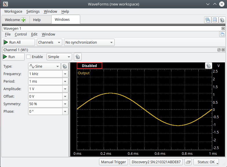
Figure 1: The Wavegen screen
The main window shows a single cycle of the waveform that will be output to the Wavegen channel 1 output pins (W1 and Gnd) when the tool is running.
You can adjust the output waveform by either typing a value or using the dropboxes on the left-side controls menu. The ‘Simple’ controls are as follows:
- Type: The type of waveform (Sine, Square, Triangle etc…)
- Frequency: The frequency of the waveform. (= 1/Period)(10MHz maximum)
- Period: The period of the waveform. (= 1/Frequency)
- Amplitude: The peak AC component amplitude of the waveform.
- Offset: The DC component that is added to the AC waveform.
- Symmetry: How symmetrical the positive and negative sides of the AC waveform are. (50% is normal)
- Phase: At what phase the waveform starts.
To output the currently displayed waveform on the corresponding output pins you need to hit the ‘Run’ Button in the upper lefthand corner. Once it is running the ‘Run’ button becomes the ‘Stop’ button.
Without hitting the ‘Run’ button you can preview what the output waveform will look like. You can go ahead and use the controls to see how each one effects the display of the waveform.
2.1.2 Scope (AD2)
The oscilloscope or “scope” is one of the most versatile and heavily used electronic measuring instruments in science, engineering, and industry. The oscilloscope earns its status as an important instrument because it neatly graphs how voltage varies as a function of time. Time varying voltage signals are not only important in electronic devices but also useful in measuring all kinds of other types of signals that are converted into an electrical signal by a transducer. A transducer is a device that converts one type of energy to another.
Learn to use the Scope tool of the Analog Discovery 2 by using the Wavegen tool as a AC voltage source that can be measured and displayed with channel 1 of the Scope tool.
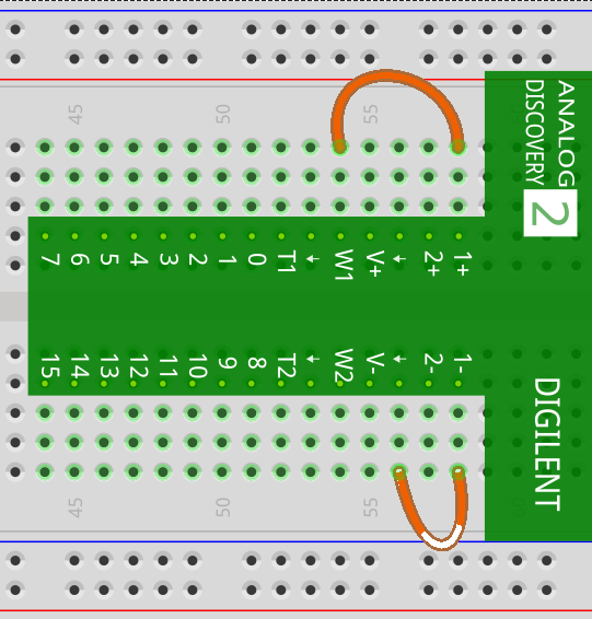
Figure 2: Connect the Wavegen (W1) to the Scope (1+)
Connect the Wavegen 1 output to the channel 1 input of the scope as shown in the circuit above by connecting the following:
Connect the Wavegen output (W1) to the positive channel 1 input (1+) of the Scope.
Connect the Wavegen output (Gnd) to the negative channel 1 input (1-) of the Scope.
From the Welcome tab in Waveforms select the Scope tool from the left-side menu and you should get a new tab that looks like the following.
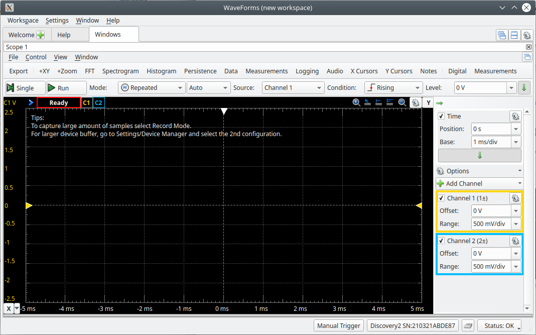
Figure 3: The Scope screen
Run the Wavegen tool to output a 1kHz sinewave at 1V amplitude and then also Run the Scope tool with its default settings. You should now have something like the following.
Note:
In Waveforms to view both the Wavegen tool and the Scope tool at the same time as shown above you can click on the middle button in the upper right hand corner of the screen when both tools are already open.

Figure 4: Split screen button
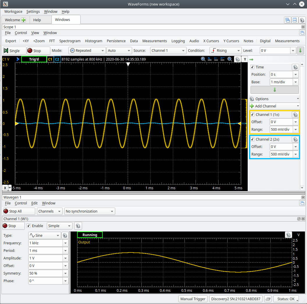
Figure 5: Scope/Wavegen split screen
A typical Oscilloscope has 3 main control sections: Vertical, Horizontal and Trigger. These controls section will be discussed in the following sections.
2.1.2.1 Vertical Section
The vertical section controls the y-axis of the displayed incoming voltage signal. There is one set of controls for every input channel. In our case since this is a 2-channel oscilloscope there are 2 sets of controls. The main vertical controls are ‘Offset’ and ‘Range’ which contribute to how the incoming waveform is displayed on the vertical/y-axis.
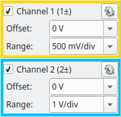
Figure 6: Vertical section controls
The key points about the vertical/y-axis are:
- There are 2 vertical channels: channel 1 in yellow and channel 2 in blue.
- The channels can be turned on and off using the checkbox next to the Channel name.
- It is the voltage axis. The higher the incoming voltage, the farther from the ‘ground’ (0 Volt level) the graph moves for a given ‘Range’ setting.
- Voltage can be positive or negative relative to ‘ground’. Positive input voltages moves the graph point above the ‘ground’; negative input voltage moves it below the ‘ground’.
Vertical Position
Each input channel has a ‘ground’ (0 Volt level) indicator on the left edge of the screen. Below is an image showing the vertical position of channel 1 which should now be in the vertical center of the display.

Figure 7: Vertical position indicator
The ‘Offset’ dropdown box or clicking and dragging the indicator will move this position indicator up and down on the display which in turn will also move the incoming voltage waveform up and down on the display.
Note:
All of the controls on the Scope have no effect on the incoming voltage it only effects the way the waveform is displayed on the screen.
Volts per Division
A typical oscilloscope will have 8-10 vertical divisions on the display. You can change the graph’s y-axis scale (usually expressed in volts per division or VOLTS/DIV) using the Range dropdown box to control how the incoming voltage waveform is scaled when it is displayed on the graph.
The displayed waveform (currently 2V peak to peak) should currently span approximately 4 vertical divisions of the oscillscope’s screen if the range is currently set to 500mV/div. When you multiply the number of vertical divisions the waveform spans (~4) by the VOLTS/DIV setting (500mV/div) you arrive at that peak to peak voltage (2Vp-p).
Adjust Vertical
Adjust the following Channel 1 vertical controls to see how they effect the Scopes graph display.
Make a change to the ‘Offset’ dropdown box to other values and see the result. It should move the waveform and the ‘ground’ indicator up and down on the screen. You can also try clicking and dragging on the indicator to see the results. Return the position back to the center of the display by setting the offset to 0V.
Make a change to ‘Range’ dropdown box and see result. It should scale the magnitude of the waveform on the screen. Return the ‘Range’ back to 500mV/div.
2.1.2.2 Horizontal Section
The horizontal section controls the x-axis, which is generally used as the time-axis. There is only one common set of controls for all of the input channel. The horizontal controls are ‘Position’ and ‘Base’ which all contribute to how the incoming waveform is displayed on the horizontal/x-axis.
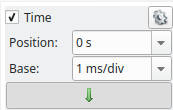
Figure 8: Horizontal section controls
The key points about the x-axis are:
- The x-axis is generally a time axis. In that mode, the point on the screen sweeps across at a constant user selectable speed, covering equal distances across the screen in equal times.
- If there is no input signal, you will see a horizontal line at y = 0, usually in the center of the display.
- Changing the ‘Base’or ’Sec/div’ changes the scale of the x-axis on the graph display.
- Time is scaled in units of seconds/division (Sec/div). To rescale the time axis, use the ‘Base’ control dropbox.
Horizontal Position
The current horizontal position is indicated on the top edge of the graph, typically in the center of the display which represents 0 seconds. This mark indicates where the current captured waveform was triggered. Below is an image showing the horizontal position of the display.

Figure 9: Horizontal position indicator
The ‘Position’ dropdown box or clicking and dragging the indicator will move this position indicator left and right on the display which in turn will also move the incoming voltage waveform left and right on the display.
Seconds per Division
A typical oscilloscope will have 10 horizontal divisions on the display. You can change the graph’s x-axis scale (expressed in seconds per division or Sec/div) using the ‘Base’ dropdown box to control how the time-base of the incoming voltage waveform is scaled when it is displayed on the graph.
Adjust Horizontal
Adjust the horizontal controls to see how they effect the Scopes graph display.
Make a change to the ‘Position’ dropdown box to other values to see the result. It should move the waveform and the position indicator left and right on the screen. You can also try clicking and grabbing the indicator to see the result. Return the position back to the center of the display by setting the ‘Position’ back to 0s.
Make a change to the ‘Base’ dropdown box to see result. It should scale the time base of how the waveform is displayed on the screen. Return the ‘Base’ back to 1ms/div.
2.1.2.3 Trigger Section
An oscilloscope’s trigger function synchronizes the horizontal sweep at the correct point of the signal, essential for clear signal characterization. Trigger controls allow you to stabilize repetitive waveforms and capture single-shot waveforms. The trigger makes repetitive waveforms appear static on the oscilloscope display by repeatedly displaying the same portion of the input signal. Imagine the jumble on the screen that would result if each sweep started at a different place on the signal, as illustrated the figure below.
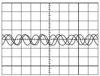
Figure 10: Example of an un-triggered sinewave
Trigger Controls

Figure 11: Trigger section controls
Along the Trigger controls toolbar you have the following controls:
Single - When the ‘Single’ button is pushed the acquisition will wait for a trigger signal to occur and then capture a single acquisition from the inputs, automatically stopping after the acquisition is complete.
Run/Stop - When the ‘Run’ button is pushed the acquisition will wait for a trigger signal to occur and then capture an acquisition from the inputs. Once the first acquisition is finished it will then wait for another trigger signal to start the next one. This will happen indefinitely until the ‘Stop’ button is pushed.
Mode: - These are more advanced settings that will not be used in this course. For our purposes they should be set to both ‘Repeated’ and ‘Auto’.
Source: - This sets which signal you wish to use to trigger the aquisition. For this course we will only use Channel 1 as the trigger source.
Condition: - This sets what type of edge you would like to trigger on: Either Rising, Falling or Both. For this course we will only use the Rising edge.
Level: - This control sets at what voltage the incoming signal (ie. Channel 1) needs to pass through in order to activate a trigger. You can also adjust this level by clicking and dragging on the trigger level indicator on the right side of the graph display.

Figure 12: Trigger level indicator
Adjust the trigger controls to see how the effect the Scopes graph display.
Adjust the triggers ‘Level’ by click and dragging the trigger level indicator up and down and see the results. Notice, if you move the trigger level above or below the peaks of the waveform what happens? The signal is no longer triggered. Use the ‘Level’ in the trigger toolbar to reset the trigger level back to 0V.
Note:
The waveform will trigger on the edge (Rising or Falling) that is selected under ‘Condition’ where the trigger level indicator intersects the horizontal ‘Position’ indicator.
2.1.2.4 Measurements
In the Scopes tools toolbar at the top of the display. We are only going to look at the ‘Measurements’ tool in this lab.

Figure 13: Scopes tools toolbar
After selecting the Measurements tab a windows will open up on the side of the graph display as shown below. You can then add measurements that will be automatically calculated from the waveform that is captured on the Scopes graph.
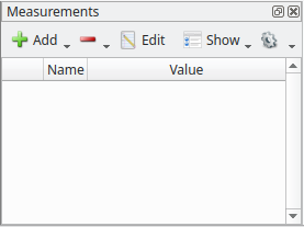
Figure 14: Measurements tool
To add a measurement use the Add dropdown and select ‘Define Measurement’. Which will give you an Add measurement selection box like shown below.
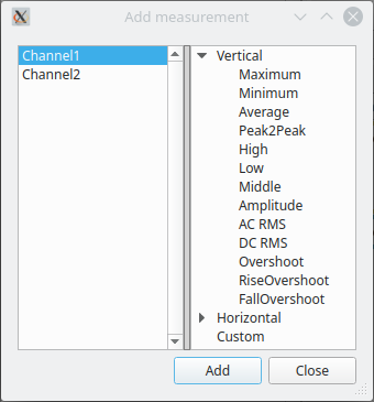
Figure 15: Measurements tool selection
Here you can select which channel you would like to make the measurement on as well as the type of measurement.
- Create a peak to peak voltage measurement for Channel 1 using the steps onlined above. Once created you should see that a measurement is being made on the incoming Channel 1 waveform with a reading about 2V. You can add as many measurements as you like.
Note:
These automatic measurements are only as good as the input waveform that you give them to do the calculations on. For example, If you are trying to obtain a voltage measurement and the signal is either really tiny on the screen or way to big for the screen (part of the waveform goes off the top of the display) the calculation will be made but could be incorrect. When making frequency or any measurement where the period of a cycle needs to be know, You need to make sure that more than a single cycle is shown.
2.1.3 Capacitance (DMM)
Use the digital multimeter to measure the capacitance of a capacitor.
- With the red banana lead connected to the (capacitor symbol) input and the black banana lead connected to the COM input on the bottom of the device rotate the control select knob to the (capacitor symbol) position as shown below.

Figure 16: Capacitance measurement
- To measure the 1uF capacitor available in your kit you simply need to connect the capacitor between the red and black alligator probes to measure the capacitance. This can be done using the breadboard or directly as shown below.

Figure 17: Capacitance measurement breadboard connections

Figure 18: Direct capacitance measurement
- Measure the capacitors available in the kit: 1.0uF, 220nF and 100nF and record your measurements on the results sheet.
2.1.4 AC Voltage (DMM)
Note:
An ideal voltmeter is an open circuit.
Use the digital multimeter and the Analog Discovery 2 to measure the AC RMS voltage of the Wavegen outputs on the Analog Discovery 2.
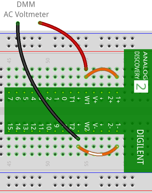
Figure 19: AC voltage measurement
Connect the circuit above using the following:
The Wavegen channel 1 (W1) from the Analog Discovery 2 as an AC voltage source. Output a Sinewave with a 100Hz frequency and a 1V amplitude.
The digital multimeter as the an AC Voltmeter. Connect the red banana lead to the (V) input and the black to the (COM) input on the bottom of the device. Rotate the control select knob to the (Vac) position as shown below.

Figure 20: DMM as an ac voltmeter
The Voltmeter Channel 1 (1+, 1-) from the Analog Discovery 2 to measure the AC RMS Voltage output of the Wavegen on the Analog Discovery 2.
Using Waveforms Wavegen tool, output the required voltages and frequencies from the results sheet. Measure and record the corresponding AC RMS voltages on both the DMM and the Analog Discovery 2 Voltmeter. The results for the first measurement are shown below.
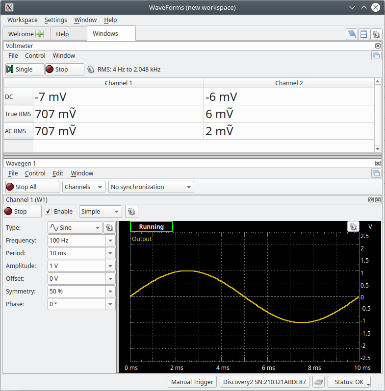
Figure 21: Voltmeter/Wavegen ac voltage measurement

Figure 22: DMM ac voltage measurement
2.1.5 AC Current (DMM)
Note:
An ideal ammeter is a short circuit.
This part just explains how to setup the DMM to measure an ac current. You won’t actually measure a current here but you will use it in the next section.
Prepare the DMM to measure an ac current.
Make sure the red banana lead is connected to the (mA) input the bottom right of the device and the black to the COM input.
Note:
Most DMM’s have multiple inputs for current so that different ranges of current can be measured accurately. This one has 2 separate inputs: One for larger currents that are less than 10 amps on the bottom left, and one on the bottom right for currents in the mA and uA ranges (internal fuse rated at 630 mA).
Figure 23: DMM current inputs
Turn the meter on by rotating the control select knob to mA (milliamps).
Make sure that the AC is displayed on the screen which indicates that you are measuring an AC current. If you try and measure a DC current in this mode the meter will display 0.00mA even if a large current is flowing.
To measure a current with a multimeter you usually need to insert the meter in series with the device you wish to measure the current through as shown below.

Figure 24: DMM current connection
Note:
When altering a circuit, like when adding an ammeter, it is good practice to turn off any power applied to the circuit while the changes are being made.
2.2 Resistor Circuit
Use a simple single resistor circuit to experiment with a AC voltage source and the AC measurement tools.
- Before connecting the circuit below use the digital multimeter as an ohmmeter to measure the resistance of the 3 resistors you will use throughout this laboratory: 220Ω, 470Ω and 1.5kΩ. Record your measurements in the appropriate place in the results sheet.

Circuit 1: AC Resistor Circuit
Click here to see a simulation demo of this circuit.Connect the circuit above using the following:
The Wavegen channel 1 (W1) from the Analog Discovery 2 as an AC voltage source. Output a Sinewave with a 500Hz frequency and a 3V amplitude.
The digital multimeter as the an AC milliammeter.
At first use a 220Ω resistor for R1 and change this resistor when required to either a 470Ω or 1.5kΩ.
The Scope Channel 1 (1+, 1-) from the Analog Discovery 2 to measure the voltage across the resistor R1.
Run the Channel 1 Wavegen and record the AC current from the DMM on your results sheet.
Use channel 1 of the Scope and the Measurements tool to obtain the following values of the voltage across the resistor: VMAX, VMIN, VAVG, VPeak2Peak and VRMS. Record your measurements on the results sheet.
Note:/
You may notice that the values you are trying to record can be difficult to obtain as the are constantly fluctuating as the Scope is continuously updating. You can either use the ‘Stop’ or ‘Single’ buttons in the upper left corner to stop the Scope from updating. Warning, you may need to push the ‘Run’ button again to obtain new values for the successive parts.
Use channel 1 of the Scope and the Measurements tool to also obtain both the frequency of the AC voltage across the resistor as well as the period. Record your measurements on the results sheet.
Now assuming that the resistor R1 is ideal we will use the math function of the scope to create a waveform of the current through the resistor R1.
- Click on ‘Add Channel’ selection box above the Vertical controls for Channels 1 and 2 and select ‘Custom’ as shown.
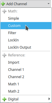
Figure 25: Add new vertical channel
ii In the popup box that opens type in ‘C1/220’. The ‘C1’ is the label for Channel 1 and we are dividing it the resistance value of 220Ω to get a new value for the current through that resistor. Also change the ‘Units:’ to A for amps. If you would like you can obtain a more accurate value for the current, use your measured value of the resistance for the calculation. Click on Ok to create the new channel.
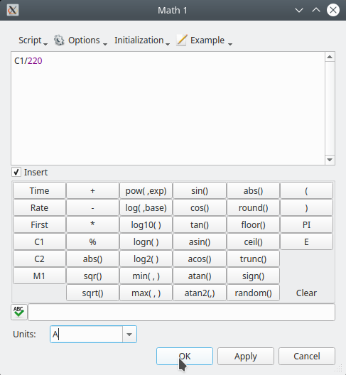
Figure 26: New math channel for current
iii The new channel will show up as ‘Math 1’ in your Vertical controls and as a Red waveform on the graph display. Adjust the ‘Range’ of the new channel to suitable one (5mA/div) where the current waveform can be seen.
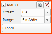
Figure 27: The new channel’s controls
Again use the Measurements tool in the Scope to calculate the RMS value of this new current waveform and record the measurement on your results sheet.
Replace the resistor (R1), first with a 470Ω resistor followed by a 1.5kΩ and repeat the same measurements as you did above making sure to record your measurements on the result sheet.
Note:
Everytime you change the resistor (R1) you need to make sure the you change the current calculation in Waveforms so that it divids by the new resistors value.
After the completion of this section turn off the ac voltage source before you modify your circuit for the next section.
2.3 Series Resistors
Use the AC measurement tools to investigate how an AC resistor voltage divider circuit operates under different source voltage frequencies.

Circuit 2: Series Resistor Circuit
Click here to see a simulation demo of this circuit.Connect the circuit above using the following:
Connect R1 and R2 in series on the breadboard.
Use the Wavegen channel 1 (W1, Gnd) on the Analog Discovery 2 as the AC voltage source.
Use the DMM to measure the frequency of the circuit by connecting it across the ac voltage source and turning the dial to Hz.
Use channel 1 (1+, 1-) and channel 2 (2+, 2-) of the Scope on the Analog Discovery 2 to measure the voltage waveforms across R1 and R2 respectively.
Enable the Wavegen as the ac voltage source in Waveforms. Set the initial sinewave to 100Hz and 3VRMS (4.243VPeak).
Use the DMM to measure the system frequency (fs) and record your measurement on the results sheet.
Use the Scope and the Measurement tool in Waveforms to to determine the RMS voltage across both resistors R1 and R2. Record your measurement on the results sheet.
Create a new channel that sums the channel 1 and channel 2 waveforms of the Scope to create the voltage source waveform (Vs).
Click on ‘Add Channel’ selection box above the Vertical controls for Channels 1 and 2 and this time select ‘Simple’.
A new math channel will be displayed as shown below. The default is the sum of Channel 1 (C1) and Channel 2 (C2) and this is what we want to obtain the source voltage.
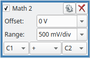
Figure 28: Voltage source channel controls
Use the controls for the new waveform to make sure it is displayed nicely of the graph.
Use the Measurements tool to measure the RMS of this new waveform (VsRMS). Record the measurement on your results sheet.
Create a new channel or modify the existing math channel from the last section where we measured current that takes the voltage across R1 (channel 1) and divids it by the resistance value (470Ω) to create the source current waveform (Is). Use the Measurements tool to measure the RMS of this new waveform (IsRMS). Record the measurement on your results sheet.
Adjust the frequency of the ac voltage source first to 1kHz and then to 10kHz while repeating all of the same measurements as above for both frequencies.
After the completion of this section just turn off the ac voltage source as you will continue to use a modified version of this circuit in the next section.
2.4 Series RC (1uF)
Use the AC measurement tools to investigate how a Series RC circuit operates under different source voltage frequencies.

Circuit 3: Series Resistor-Capacitor Circuit (1uF)
Click here to see a simulation demo of this circuit.Modify the circuit from the previous section by replacing the 220Ω resistor (R2) with an 1uF capacitor (C1).
Using the same procedures from the previous section obtain the results for the new circuit including: the system frequency, the RMS voltages for the source, the resistor and the capacitor and the circuits RMS current. Obtain the measurements for the 4 different frequencies: 100Hz, 338.6Hz, 1.0kHz and 10kHz. Record the measurements on your results sheet.
Note:
At the frequency of 338.6Hz the resistance of the resistor (470Ω) will approximately equal the reactance of the capacitor.
After the completion of this section just turn off the ac voltage source as you will continue to use a modified version of this circuit in the next section.
2.5 Series RC (100nF)
Investigate how the capacitance value of the Series RC circuit effects how the Series RC circuit operates under.

Circuit 4: Series Resistor-Capacitor Circuit (100nF)
Click here to see a simulation demo of this circuit.Modify the circuit from the previous section by replacing the 1uF capacitor (C1) with an 100nF capacitor (C2).
Using the same procedures from the previous section obtain the results for the new circuit including: the system frequency, the RMS voltages for the source, the resistor and the capacitor and the circuits RMS current. Obtain the measurements for the 4 different frequencies: 100Hz, 1.0kHz, 3.386kHz and 10kHz. Record the measurements on your results sheet
Note:
At the frequency of 3.386kHz the resistance of the resistor (470Ω) will approximately equal the reactance of the capacitor.
After the completion of this section just turn off the ac voltage source as you will continue to use a modified version of this circuit in the next section.
2.6 Series RL
Use the AC measurement tools to investigate how a Series RL circuit operates under different source voltage frequencies.
- Before connecting the circuit below use the digital multimeter as an ohmmeter to measure the resistance of the non-ideal inductor. Record your measurement in the appropriate place in the results sheet.

Circuit 5: Series Resistor-Inductor Circuit (10mH)
Click here to see a simulation demo of this circuit.Modify the circuit from the previous section by replacing the 100nF capacitor (C1) with an 10mH inductor (L1).
Using the same procedures from the previous section obtain the results for the new circuit including: the system frequency, the RMS voltages for the source, the resistor and the capacitor and the circuits RMS current. Obtain the measurements for the 4 different frequencies: 100Hz, 1.0kHz, 7.480kHz and 10kHz. Record the measurements on your results sheet
Note:
At the frequency of 7.480kHz the resistance of the resistor (470Ω) will approximately equal the reactance of the inductor.
After the completion of this section you can turn off the ac voltage source and disconnect your circuit.
2.7 Cleanup
Congratulations, you have completed the experimental part of the the laboratory. Before cleaning up, I’d suggest going through your results to check that you have completed everything and that your results make sense. If you find any issues, I’d suggest resolving or making a note of it now. If you are not continuing to work with the equipment please disconnect everything and put it away to prevent it from getting damaged.
3 Results
The following is what you are expected to complete and submit for grading for Lab 3 before the deadline:
The completed Lab 3 - Results sheet template provided at the beginning of this lab manual under Equipment required. This sheet should include the following:
- Your name, student ID and CCID.
- All of the required measurements from the lab procedures.
- All of the required calculations as discussed below.
- The required plots as discussed below.
The Lab 3 - Results sheet needs to be submitted to the Submit (Lab 3 - Results) link on eClass as a pdf document .
- Complete the online Quiz (Lab 3 - Post Lab) on eClass.
3.1 Calculations
For these calculation you only need to provide the answers in the space provided on your results sheet, you do not need to show your work.
For the Resistor Circuit calculate the resistance of each circuit by using the appropriate voltage and current measurements.
For the Series Resistors circuit calculate the resistance for each resistor: R1 and R2 for each frequency value using the appropriate voltage and current measurement.
For the Series RC (1uF) and Series RC (100nF) circuits use the appropriate voltage and current measurement to determine the resistance of the resistor and reactance of the capacitor at each frequency. From the calculated reactance value also calculate the capacitance of the capacitor at each frequency.
For the Series RL (10mH) circuit use the appropriate voltage and current measurement to determine the resistance of the resistor and the reactance of the inductor at each frequency. From the calculated reactance value also calculate the inductance of the inductor at each frequency.
3.2 Plots
To create your plots you can use whichever software you would like (Excel, Matlab, etc), export your plot as an image and import it into your Lab 3 - Results sheet in the appropriate place.
Your plots should include:
- A Plot title
- Label your axes and show what unit of measure is used.
- Include a marking for your datapoints.
- Include a line between your datapoints in the same series.
- Include a legend.
- Make sure your scales are appropriate and visible.
- Impedance-Frequency Plot: For the 5 components used in the 4 series circuits: 220Ω, 470Ω, 1uF, 100nF and the 10mH. Plot each components impedance vs. frequency on the same plot. Use a logarithmic scale for both the x-axis and y-axis.
3.3 Questions
Complete the online Quiz (Lab 3 - Post Lab) on eClass.