Lab 1: Intro to DC Circuits
ECE202 - Electrical Circuits I
Electrical and Computer Engineering - University of Alberta
1 Objectives
In this first lab session, you will become familiar with some of the common electrical tools and components used for circuits and use them to experimentally test and confirm the validity of concepts taught in the lectures. The objectives are as follows:
Introduce the following devices:
- DC Voltage and DC Current Sources
- Resistors and a Potentiometer
- DC Voltmeter, DC Ammeter and an Ohmmeter
- A Breadboard
Introduce the following concepts:
- Ohm’s Law
- Power Dissipation of a Resistor
- Kirchhoff’s Laws - (KVL and KCL)
- Series/Parallel Resistors
- Voltage/Current Dividers
- The Loading Effect - Voltmeter and Ammeter Loading
1.1 Equipment Required
- The Lab 1 - Results sheet to record your measurements.
- A Computer with Waveforms installed
- Analog Discovery 2
- Breadboard Breakout for the Analog Discovery 2 with a Ribbon Cable
- A USB A to Micro-B cable
- Digital Multimeter
- MB102 breadboard
- DC Current Source
- Jumper Wires
- 1kΩ pot
- The following Resistors (1/4 watt, 1% or 5%)
- 10Ω
- 20Ω
- 100Ω
- two 470Ω
- 1kΩ
- 4.7kΩ
- 20kΩ
- two 10MΩ
1.2 Background
2 Procedures
2.1 Equipment Familiarization
2.1.1 Resistors
A resistor is a passive electrical component to create resistance in the flow of electric current. They can be found in almost all electrical networks and electronic circuits.
The unit of measure for resistance is Ohms (Ω) in the International System of Units (SI). The Ohm is the resistance of a conductor such that a constant current of one ampere in it produces a voltage of one volt between its ends.
Therefore the current is proportional to the voltage across the conductors terminal ends. This ratio is represented by Ohm’s law:
\[I = \frac{V}{R}\] Where:
- I = the current through the conductor in amperes.
- V = the voltage across the conductor in volts.
- R = the resistance of the conductor in Ohms.
Resistors are used for many purposes. A few examples include to limit electric current, voltage division, heat generation, matching and loading circuits, control gain, and fix time constants. They are commercially available with resistance values over a range of more than nine orders of magnitude. There size and power ratings very greatly as they can be very large when used as electric brakes to dissipate kinetic energy from electric trains, or be smaller than a square millimeter for use in a smartphone.
More information - Wikipedia - Resistor

Figure 1: Fixed resistor schematic symbol (ANSI left, IEC right)
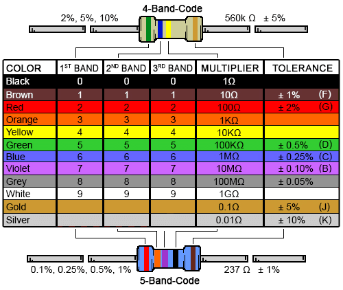
Figure 2: Resistor color codes
Note:
The last band notes the tolerance of the resistor which means that the actual resistance value can be slightly different then the rated one by that percentage over its operating temperature range.
2.1.2 Potentiometer
A potentiometer is a manually adjustable variable resistor with 3 terminals. The two outer terminals are connected to both ends of a resistive element, and the middle terminal connects to a sliding contact, called a wiper, moving over the resistive element. The resistive element can be seen as two resistors in series where the sum is the “potentiometer resistance rating”, where the wiper position is the dividing point between the first resistor and the second resistor.
More information - Wikipedia _Potentiometer

Figure 3: Potentiometer schematic symbol (ANSI left, IEC right)
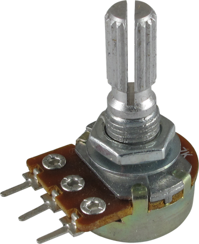
Figure 4: Potentiometer
2.1.3 Breadboard
A breadboard is a rectangular board with regular spaced holes for easily creating electrical connections between electronic components, a typical one is shown below. Due to the easy assembly of electrical connections these boards are mostly used to prototype circuits however they do have their limitations (ie. higher frequency design). The connections aren’t permanent and they can be removed and placed again and again.
The breadboard will be used to build the basic circuits used in these labs.
The vertical columns comprising of a pair of 5 interconnected holes are called terminals, while the 4 horizontal long rows are called power rails; These power rails are mostly used to connect the power supplies to the breadboard and are marked by red and blue lines in the image below and forming 4 separate groups of interconnected holes.
The reason it’s called a breadboard dates back to when electronics components were much bigger and people would actually use wooden breadboards (boards used to cut bread) to connect electronic circuits. Fortunately, things have changed since then and only the name has been retained.
More information - Wikipedia Breadboard

Figure 5: Anatomy of a Breadboard
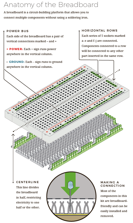
Figure 6: Typical breadboard
If you haven’t already. Please connect the metal plate to the back of breadboard, this metal plate is there for 2 reasons: The first is to act as a backing for when you push components into the holes of the breadboard so they don’t pierce the paper backing that is holding the metal contacts in place. The second is it acts as a shielding to prevent electrical noise from emitting or entering your circuits.

Figure 7: Breadboard without backing

Figure 8: Breadboard with backing
2.1.4 Analog Discovery 2
The Digilent Analog Discovery 2™, developed in conjunction with Analog Devices®, is a multi-function instrument that allows users to measure, visualize, generate, record, and control mixed signal analogue and digital circuits. The low-cost Analog Discovery 2 is small enough to fit in your pocket, but powerful enough to replace a stack of lab equipment, providing engineering students, hobbyists, and electronics enthusiasts the freedom to work with analogue and digital circuits in virtually any environment, in or out of the lab.
2.1.4.1 Software Installation
Install the required software Waveforms for your operating system.
Figure 9: Waveforms logo
2.1.4.2 Connections
Connect the Analog Discovery 2.
- Use the provided USB A to micro-B cable to connect your Analog Discovery 2 to the USB port on your computer.

Figure 10: Analog Discovery 2 connected to a computer
- Connect the one end of the ribbon cable with the notch in the proper orientation to the Analog Discovery 2 as shown below. Then connect the other end of the ribbon cable to the Breadboard Breakout using the supplied 15x2 header pins. Make sure that the orange wires of the ribbon cable end up on the same side as the breadboard breakout pin labeled 1+.

Figure 11: Connecting the breakout board to the Analog Discovery 2
- Plug the breadboard breakout into the breadboard as a shown.

Figure 12: Breakout board connected to the breadboard
2.1.4.3 DC Power Supply
Use the DC Power Supply on the Analog Discovery 2.
- Start the ‘Waveforms’ software for the first time.
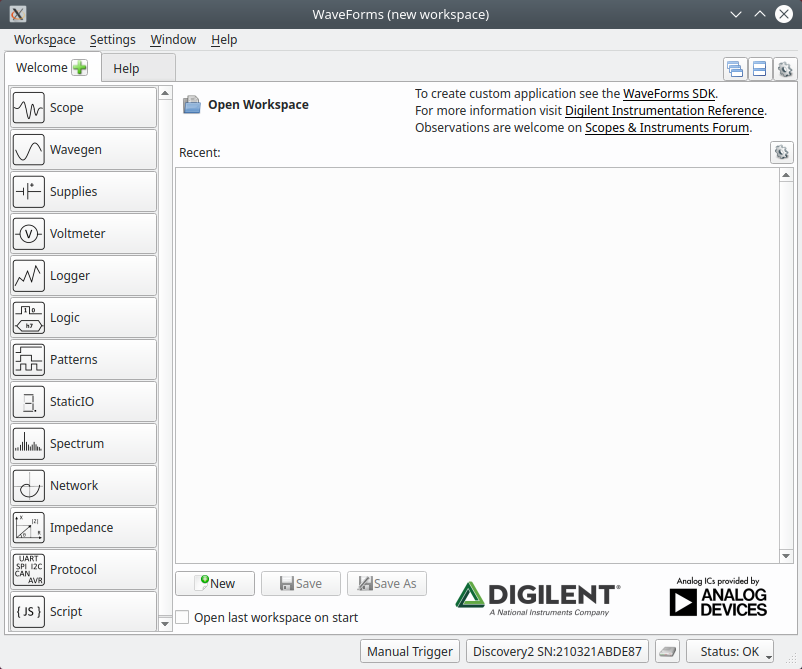
Figure 13: Waveforms start screen
If everything is connected and installed correctly you should notice the device and serial number (SN:) in the bottom corner as well as the devices status (OK).
The first tab displayed should be the welcome screen. All of the available tools on the device are located along the left side of this tab. Click on the “Supplies” button and a new tab will open with the controls for the Supplies.
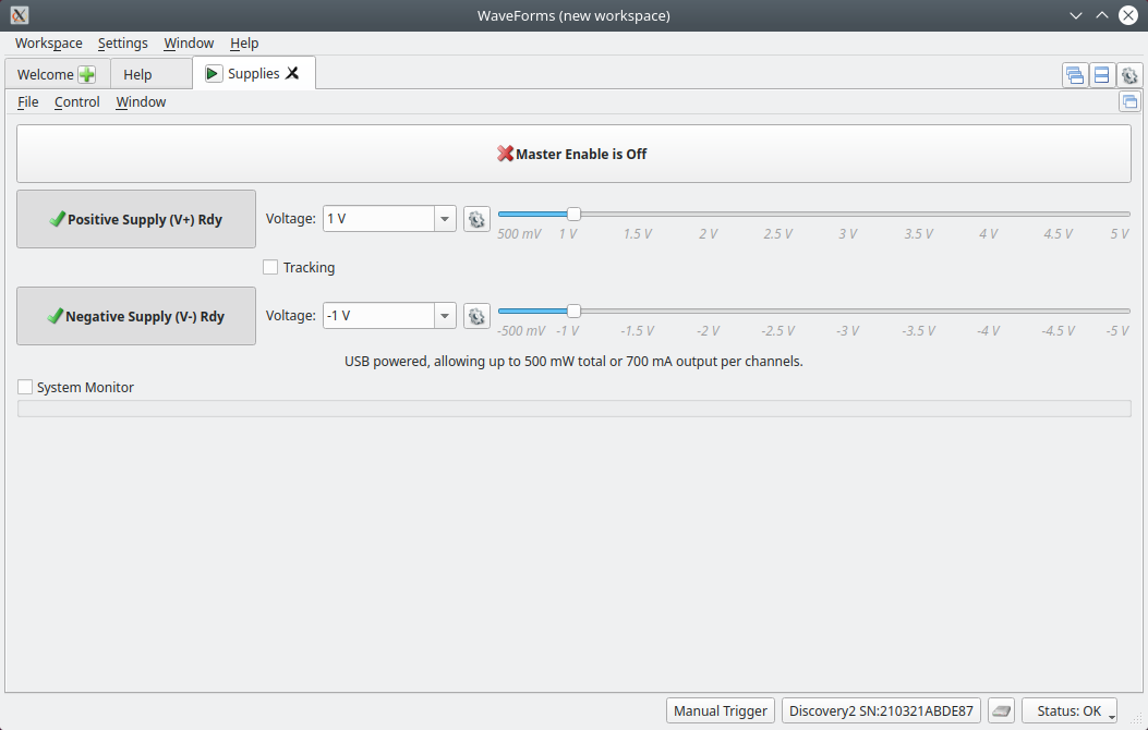
Figure 14: Waveforms DC power supply control screen
The Analog Discovery 2 is equipped with two DC power supplies: 1 positive supply and 1 negative supply.
Both power supplies should currently be disabled as the “Master Enable is Off”.
By clicking on the “Master Enable” both supplies will then output the corresponding voltage for that supply on it’s designated output pins: (V+ and Gnd/) and (V- and Gnd/) for the positive and negative supplies respectively.
Note:
On the Analog Discovery 2 they show the circuit ground or circuit common of the device with a down arrow (), it can also be abbreviated as Gnd. There are 4 of these on the Analog Discovery 2 and they are all a common ground node.Each supply has its own enable as well.
To control the output voltage of the supply you can either use the drop down to select a voltage, type the number to 3 decimal places or use the slider. The positive V+ has a range from 500mv to 5.0V while the Negative V- is from -500mv to -5.0V
There is also a “Tracking” checkbox, when this is enabled the positive and negative voltage will always have the same absolute value. In this mode you can use any of the controls to set both output voltages.
Go ahead and play with the Supplies controls to test them out to see how they function.
2.1.4.4 Voltmeter
Use the Voltmeter on the Analog Discovery 2 to measure the output of the voltage supply on the Analog Discovery 2
- Use 2 jumper wires to make the following connections on the
breadboard.
- V+ to 1+
- Gnd/ to 1-
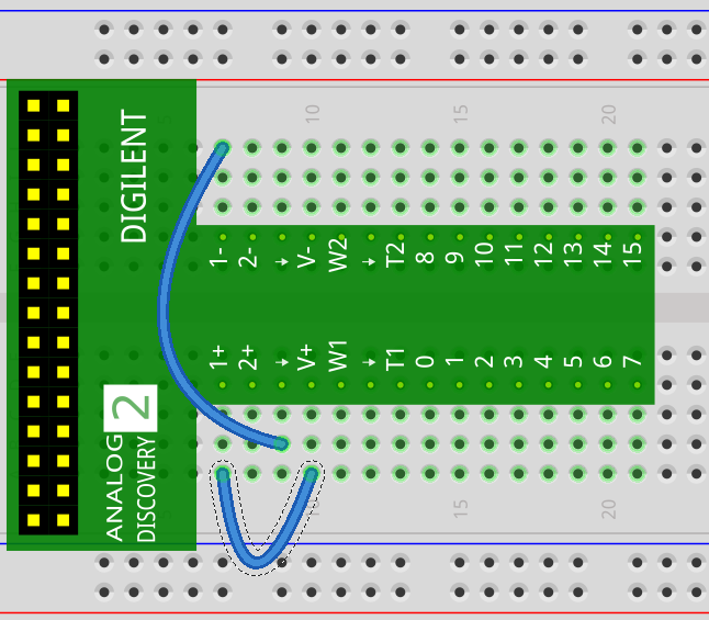
Figure 15: Breadboard connections to measure V+ on Channel 1
- From the Welcome screen start the “Voltmeter” tool to open the controls for the Voltmeter.
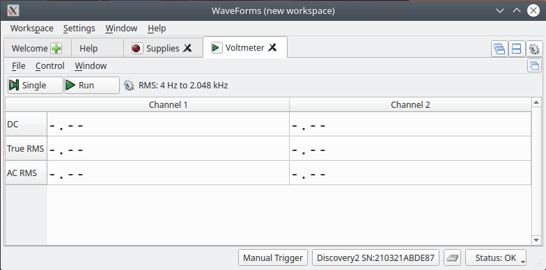
Figure 16: Waveforms voltmeter screen
The Analog Discovery 2 is equipped with 2 voltmeters: Channel 1 and Channel 2.
Both voltmeters should currently be disabled as they are not running.
By clicking on the “Run” button both voltmeters will then display the corresponding voltage that is currently measuring on its input pins: (1+ and 1-) and (2+ and 2-) for Channel 1 and Channel 2 respectively. The measurements are updated at a certain refresh rate continuously.
Hitting the same button again, now “Stop”, will stop the acquisitions.
There is also a “Single” acquisition button that will acquire a single measurement and then stop on its own.
With each acquistion there are 3 values that are calculated: DC, True RMS, AC RMS. The reading we will use for this lab is the DC reading. You will learn what the difference of these readings are later in this course.
Using both the “Supplies” and “Voltmeter” controls see if you can generate a voltage using the positive supply and measure it using channel 1 of the voltmeter. Try changing the voltage and measuring again. Play with all of the “Supplies” and “Voltmeter” controls until you are familiar with them.
Note
You can enable or disable a tool from the tab by clicking on the green triangle to enable and the red square to disable.- Use 2 jumper wires to make the following connections on the
breadboard.
2.1.5 Digital Multimeter (DMM)
A digital multimeter is a test tool used to measure electrical quantities, principally: voltage (volts), current (amps) and resistance (Ohms). It is a standard diagnostic tool for engineers in the electrical/electronic industries.
Digital multimeters long ago replaced needle-based analog meters due to their ability to measure with greater accuracy, reliability and increased impedance.
Digital multimeters combine the testing capabilities of single-task meters; ie. the voltmeter (for measuring volts), ammeter (amps) and ohmmeter (Ohms). Often, they include several additional specialized features or advanced options. Engineers with specific needs, therefore, can seek out a model targeted to meet their needs.
The face of a digital multimeter typically includes four components:
- Display: Where measurement readouts can be viewed.
- Buttons: For selecting various functions; the options vary by model.
- Dial (or rotary switch): For selecting primary measurement values (volts, amps, Ohms).
- Input jacks: Where test leads are inserted.

Figure 17: A typical digital multimeter (DMM)
2.1.5.1 Resistance Measurement
Prepare the digital multimeter (DMM) to measure a resistor.
- If you haven’t installed the battery in your DMM, please do this first. You will need an appropriate screw driver to remove the back cover to install the provided 9V battery.

Figure 18: Placing a battery in the DMM
Connect a red banana lead to the Ω input on the bottom right of the device.
Connect a black banana lead to the COM input on the bottom of the device.
Turn the meter on by rotating the control select knob to Ω (ohmmeter).
When nothing is connected between the red and black banana leads it should display OL indicating an open circuit or infinite resistance.
When you connect (short) the red and black test leads ends together it should display approximately 000.0 indicating a short circuit or zero resistance.

Figure 19: Measuring zero ohms when test leads are shorted
- Connect the red and black alligator clips to the appropriate test lead as this will make it easier to measure the resistances in the next part.

Figure 20: Alligator clips connecting to the test leads
Use the resistor color code chart above to find the resistance values in the chart below. Write the color bands required for each resistor value and write the colors on the results page. Then use the digital multimeter to measure the actual resistance value of each resistor and record it on your results sheet. To measure the resistance connect the red and black alligator clips to either end of the resistor. These are the resistors that you will use throughout this first lab so keep them handy.
| R1 | R2 | R3 | R4 | R5 | R6 |
|---|---|---|---|---|---|
| 10 | 100 | 470 | 1k | 4.7k | 10M |

Figure 21: Measuring a 470Ω Resistor
Measure resistors in series.
Table 2: Measure series resistors
RS1
RS2
RS3
100 + 470
1k + 4.7k
10M + 10M
Use the breadboard to place the resistors in the table above in series as shown in the image below.

Figure 22: Resistor symbols connected in series

Figure 23: Series resistors connected on a breadboard
Use the alligator clips on the leads of the resistors to measure the effective resistance of the two components in series and record your measurements on your result sheet.
Measure resistors in parallel.
Table 3: Measure parallel resistors
RP1
RP2
RP3
100 // 470
1k // 4.7k
10M // 10M
Use the breadboard to place the resistors in the table above in parallel as shown in the image below.

Figure 24: Resistors symbols connected in parallel

Figure 25: Parallel resistors connected on a breadboard
Use the alligator clips on the leads of the resistors to measure the effective resistance of the two components in parallel and record your measurements on your results sheet.
2.1.5.2 DC Voltage Measurement
Note:
An ideal voltmeter is an open circuit.
Use the digital multimeter (DMM) to measure a dc voltage.
Prepare the DMM to measure a DC voltage.
Make sure the red banana lead is connected to the V input the bottom right of the device.
Make sure the black banana lead is connected to the COM input on the bottom of the device.
Turn the meter on by rotating the control select knob to V (voltmeter).
Press the function button (FUNC) until DC is selected at that top of the screen.

Figure 26: DC function indication on the DMM
Connect the DC voltmeter to the Analog Discovery 2 positive supply using either header pins or jumper wire:
Connect the red probe of the DMM to V+.
Connect the black probe of the DMM to Gnd.

Figure 27: DC voltmeter connected to the breadboard
Enable the positive supply in Waveforms, the output voltage should be displayed on the DMM. Now change the output voltage in Waveforms and make sure that your DMM is updated to correspond to this new setting.
Disable the voltage supply in Waveforms and the DMM should now read close to 0V.
Disconnect the DMM from the breadboard.
2.1.5.3 DC Current Measurement
Note:
An ideal ammeter is a short circuit.
This part just explains how to setup the DMM to measure a DC current. You won’t actually measure a current here but you will use it in the next section.
Prepare the DMM to measure a DC current.
Make sure the red banana lead is connected to the (mA) input the bottom right of the device and the black to the COM input.
Note:
Most DMM’s have multiple inputs for current so that different ranges of current can be measured accurately. This one has 2 separate inputs: One for larger currents that are less than 10 amps on the bottom left, and one on the bottom right for currents in the mA and uA ranges (internal fuse rated at 630 mA).
Figure 28: DMM current inputs (left = 10AMAX, center = common, right = 630mAMAX
Turn the meter on by rotating the control select knob to mA (milliamps).
Press the function button (FUNC) until DC is selected at that top of the screen.
To measure a current with a multimeter you usually need to insert the meter in series with the device you wish to measure the current through as shown below.

Figure 29: DMM current measurement connection (needs to be in series with component)
Note:
When altering a circuit, like when adding an ammeter, it is good practice to turn off any power applied to the circuit while the changes are being made.
2.2 Ohm’s Law and Power
Ohm’s Law
The current through a resistor in amps (A) is equal to the voltage across the resistor (V) divided by the resistance of the resistor R in Ohms (Ω):
\[I = \frac{V}{R}\]
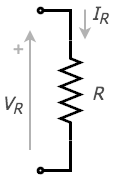
Figure 30: A Resistor (R) with its voltage and current polarity
Power Dissipated in Resistors
Any resistance in a circuit that has a current flowing through it dissipates power. This electrical power is converted into heat energy and this is why resistors have a power rating. This rating is the maximum power that can be dissipated from the resistor without it burning out. The rate at which the electrical energy is converted to heat is the power of dissipation.
\[P = I_R^2 \cdot R\]
Experiment with the concepts of both Ohm’s Law and Power Dissipated in Resistors by connecting the circuit below and following the required procedures.

Circuit 1: Ohm’s law circuit
Click here to see a simulation demo of this circuit.Connect the circuit above using the following:
Use the Positive DC Voltage Supply from the Analog Discovery 2 as VS. (V+ and Gnd/)
Use the Voltmeter from the Analog Discovery 2 to measure VR. (1+ and 1-)
Use the DMM as a milli-ammeter to measure IR. You might want to use header pins to connect the DMMs probes to the breadboard.
At first use a 470Ω resistor for R1 and then change this resistor when required to either the 1.0kΩ or the 4.7kΩ.
It should look something like this when completed.

Figure 31: Ohm’s law circuit shown on breadboard
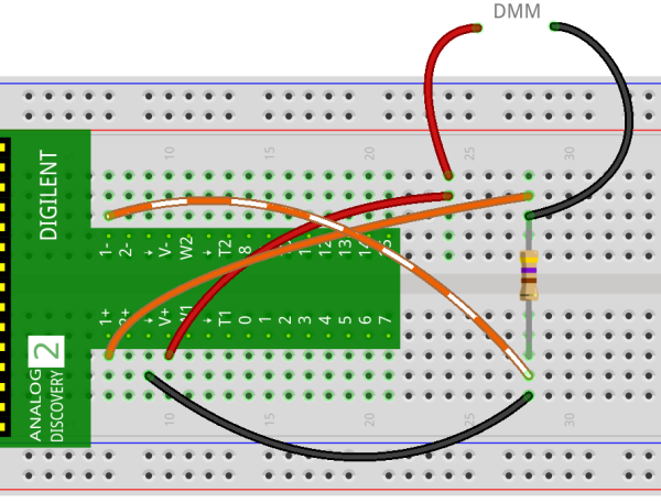
Figure 32: Ohm’s law circuit (same as breadboard)
Turn on the Analog Discovery 2 positive voltage source and adjust it to 5V.
Measure and record on your results sheet the current through and the voltage across the resistor with the following voltages applied. (5V, 3.5V, 1V, 0V, -2.5V, -5V)
For 0V simply disable the voltage supply.
For the negative voltages move the one end of the jumper wire that connects to the V+ output of the Analog Discovery 2 to the V- output and use the negative supply controls in Waveforms to adjust the voltage.
Note:
Both the voltage and current should be positive when you apply a positive voltage and both should be negative when you supply a negative voltage. If this is not the case you need to interchange the leads either on the DMM or the voltmeter so the correct sign is displayed.Try replacing the resistor with first a 1.0kΩ and then a 4.7kΩ and repeat the same measurements as above for each resistor making sure to record your results.
Once all of the required measurements are obtained and checked, turn off the Analog Discovery 2 voltage sources and disconnect the circuit.
2.3 Voltage Divider
Kirchhoff’s Voltage Law
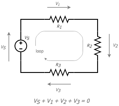
Figure 33: Kirchoffs voltage law (KVL)
Kirchhoff’s Voltage Law (KVL) is one of his fundamental laws we can use for circuit analysis. His voltage Law states that for a closed loop series path the algebraic sum of all the voltages around any closed loop in a circuit is equal to zero. This is because a circuit loop is a closed conducting path so no energy is lost.
In other words the algebraic sum of ALL the potential differences around the loop must be equal to zero as: \(\Sigma V = 0\). Note here that the term “algebraic sum” means to take into account the polarities and signs of the sources and voltage drops around the loop.
This idea by Kirchhoff is commonly known as the Conservation of Energy, as moving around a closed loop, or circuit, you will end up back to where you started in the circuit and therefore back to the same initial potential with no loss of voltage around the loop. Hence any voltage drops around the loop must be equal to any voltage sources met along the way.
Experiment with Kirchhoff’s Voltage Law by connecting the circuit below and following the required procedures.

Circuit 2: Voltage divider circuit
Click here to see a simulation demo of this circuit.Connect the circuit above using the following:
Use the positive DC voltage supply from the Analog Discovery 2 as VS. (V+ and Gnd/)
Use voltmeter channels 1 and 2 from the Analog Discovery 2 to measure VS and V1 respectively. Use channel 1 to measure V2 as well, you will need to move the channel 1 wires back and forth when required depending on which measurement is needed.
Use the DMM as a milli-ammeter to measure IS. You might want to use header pins to connect the DMM probes to the breadboard.
Use a 470Ω resistor for R1.
At first, use a 100Ω resistor for R2 and change this resistor when required to either a 470Ω, 1.0kΩ or 4.7kΩ.
It should look something like this when completed.

Figure 34: Voltage divider circuit shown on breadboard
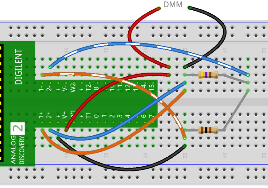
Figure 35: voltage divider circuit (same as breadboard)
Turn on the Analog Discovery 2 positive voltage source and adjust it to 5V.
Measure and record the current through (IS) and the 3 voltages: the source voltage (VS), across resistor R1 (V1) and across resistor R2 (V2).
Replace the resistor (R2), first with a 470Ω resistor followed by a 1kΩ and 4.7kΩ and repeat the same measurements as above making sure to record your results.
Once all of the required measurements are obtained and checked, turn off the Analog Discovery 2 voltage sources and disconnect the circuit.
2.4 Current Divider
Kirchhoff’s Current Law
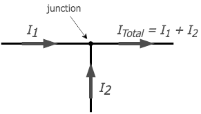
Figure 36: Kirchoffs current law (KCL)
Kirchhoff’s Current Law (KCL) is another one of the fundamental laws used for circuit analysis. His current law states that for a parallel path the total current entering a circuit’s junction is exactly equal to the total current leaving the same junction. This is because it has no other place to go as no charge is lost.
In other words the algebraic sum of ALL the currents entering and leaving a junction must be equal to zero as: \(\Sigma I_{IN} = \Sigma I_{OUT}\).
This idea by Kirchhoff is commonly known as the Conservation of Charge, as the current is conserved around the junction with no loss of current.
Test the current source by connecting the circuit below and following the required procedures.
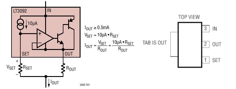
Figure 37: LT3092 (left = internal circuit, right = package pinout
Configure the LT3092 above on the breadboard as a 10mA current source using the following:
The LT3092 current source.

Figure 38: LT3092 shown mounted on pcb for use on breadboard
A 20kΩ resistor as Rset at pin 1 (Set) of the device
A 20Ω resistor as Rout at pin 2 (Out) of the device, the other ends of both Rset and Rout need to get connected together.
Pin 3 (IN) of the device needs to get connected to the V+ of the Analog Discovery 2.
Connect the red probe of the DMM configured as a milli-ammeter to the Iout point in the diagram above. Connect the black probe to the V- pin of the Analog Discovery 2.
Your circuit should look something like this when completed.

Figure 39: Current source circuit shown on breadboard
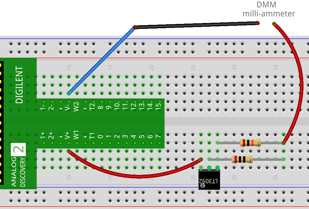
Figure 40: Current source circuit (same as breadboard)
- Turn on both the positive and negative voltage supplies on the Analog Discovery 2 and you should get an approximate reading of 10mA on the DMM.
Experiment with Kirchhoff’s Current Law by connecting the circuit below and following the required procedures.

Circuit 3: Current divider circuit
Click here to see a simulation demo of this circuit.Connect the circuit above using the following:
Use the 10mA current source you connected in the previous step.
Use the voltmeter channel 1 on the Analog Discovery 2 to measure VS.
Use the DMM as a milli-ammeter to first measure IS. You will then need to reconfigure your circuit slightly to obtain the I1 and I2 measurements when required.
Use a 470Ω resistor for R1.
At first use a 100Ω resistor for R2 and change this resistor when required to either a 470Ω, 1.0kΩ or 4.7kΩ.
It should look something like this when completed.
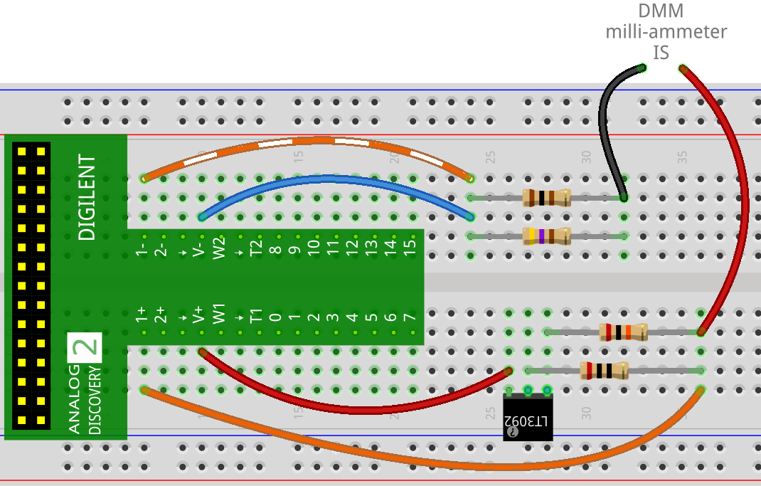
Figure 41: Current divider circuit - Measuring IS
Turn on both the positive and negative voltage supplies on the Analog Discovery 2 to 5.0V and -5.0V and you should get an approximate reading of 10mA on the DMM for IS.
Measure and Record both the IS value from the DMM and the VS reading from Waveforms. To obtain the IS and VS measurements for the other values of resistor (R2) first replace with a 100Ω resistor with a 470Ω followed by a 1kΩ and 4.7kΩ and repeat these measurements and record your results.
To obtain a measurement for I1 you will need to reconfigure your circuit so the multimeter is in the new position. It should look something like this when completed.
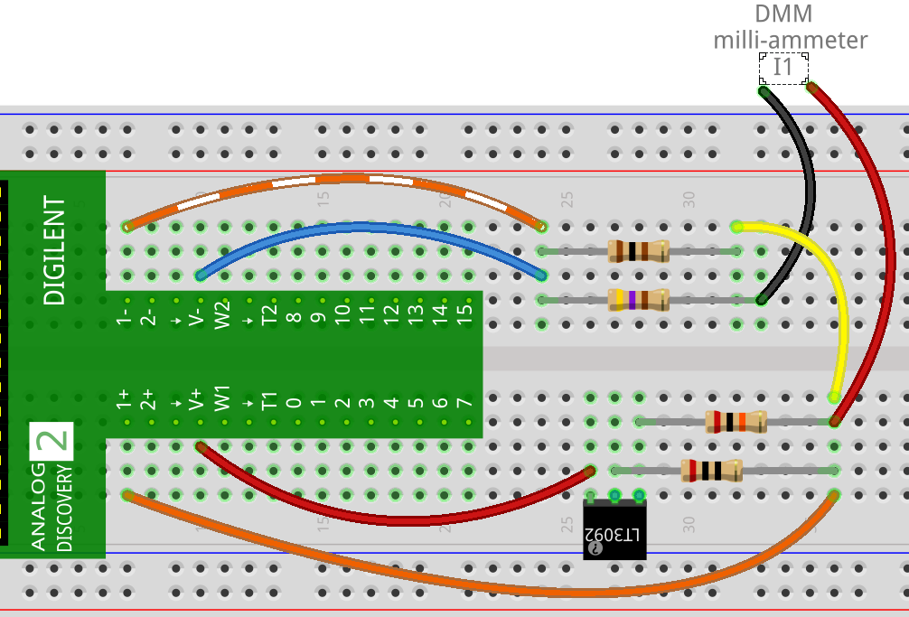
Figure 42: Current divider circuit - Measuring I1
Measurement and record the values for I1 for each of the 4 resistors (100Ω, 470Ω, 1.0kΩ, 4.7kΩ) taking their turn as R2.
To obtain a measurement for I2 you will again need to reconfigure your circuit so the multimeter is in the new position. It should look something like this when completed.
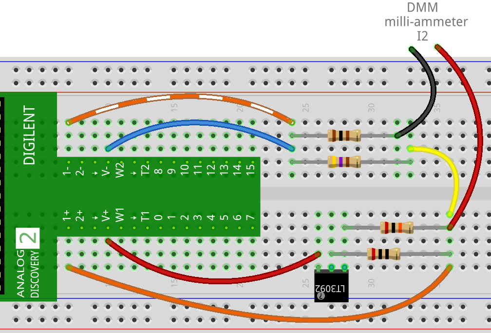
Figure 43: Current divider circuit - Measuring I2
Now measurement and record the values for I2 for each of the 4 resistors (100Ω, 470Ω, 1.0kΩ, 4.7kΩ) taking their turn as R2.
Once all of the required measurements are obtained and checked, turn off the Analog Discovery 2 voltage sources and disconnect the circuit.
2.5 Potentiometer Divider
Experiment with a Potentiometer by connecting the circuit below and following the required procedures.

Circuit 4: Potentiometer divider circuit
Click here to see a simulation demo of this circuit.Connect the circuit above using the following:
Use the Analog Discovery 2 positive voltage source as VS.
Use both Analog Discovery 2 voltmeters to measure the voltage across each part of the potentiometer: V1 and V2.
Use the DMM as an ammeter to measure IS.
Use the 1.0kΩ potentiometer.
The circuit should look something like this when completed.
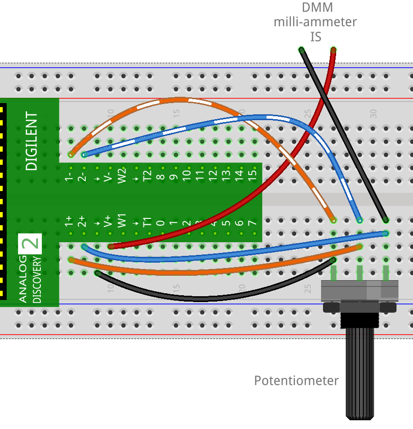
Figure 44: Potentiometer divider circuit
Turn on the Analog Discovery 2 voltage source and adjust it to 5V.
Turn the potentiometer knob until you obtain the V1 setpoints of (0V, 1V, 2V, 2.5V, 4V, 5V) making sure to measure and record the values of V1, V2, and I1 at each point.
Once all of the required measurements are obtained and checked, turn off the Analog Discovery 2 voltage sources and disconnect the circuit.
2.6 Loading Effect
Loading Effect
The loading effect is to what degree a measurement device impacts the electrical properties of the circuit under test (ie. voltage, current, resistance). Ideally the piece of equipment will have a negligible effect on the circuit and therefore give you the correct readings. However, under certain conditions the measurement device can have significant effect and alter the normal operation of the circuit and therefore give your readings an unexpected result if not accounted for.
2.6.1 Voltmeter Loading
Voltmeter Loading
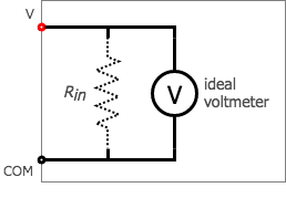
Figure 45: Non-ideal voltmeter
An ideal voltmeter imposes no load on the circuit being measured so as to not disturb the circuit. In practice, voltmeters draw some current and hence some small amount of load to the circuit affecting results.
So in an ideal voltmeter, the resistance of the meter is infinite.
In practice, voltmeters originally had resistance of several thousand Ohms, 30KΩ or 100KΩ was common. The resulting power used was required to deflect a moving needle galvanometer type meter.
Later electronic meters with input amplifiers such as vacuum tube and transistorized volt meters drew much less current with very high impedance and active amplifiers to drive the meter movements; today’s digital multimeters typically have 10MΩ input impedance.
Experiment with Voltmeter Loading Circuit by connecting the circuit below and following the required procedures.

Circuit 5: Voltmeter loading circuit
Click here to see a simulation demo of this circuit.Connect the circuit above using the following:
Use the Aanlog Discovery 2 as the voltage source VS
Use the DMM as the Non-Ideal Voltmeter to measure the voltage across R2.
Use two 10MΩ resistors in series as R1 and R2.
Turn on the Analog Discovery 2 voltage source and adjust it to 5V.
With the Non-ideal Voltmeter across (R2) measure and record the voltage.
Move the Non-ideal Voltmeter to measure the voltage across (R1) and record the voltage again.
Now move the Non-Ideal Voltmeter to measure the voltage across (VS) and record the voltage reading once again.
Once all of the required measurements are obtained and checked, turn off the Analog Discovery 2 voltage source and disconnect the circuit.
2.6.2 Ammeter Loading
Ammeter Loading
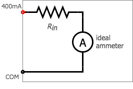
Figure 46: Non-ideal ammeter
Just like voltmeters, ammeters tend to influence the amount of current in the circuits they’re connected to. However, unlike the ideal voltmeter, the ideal ammeter has zero internal resistance, so as to drop as little voltage as possible as electrons flow through it. Note that this ideal resistance value is exactly opposite as that of a voltmeter. With voltmeters, we want as little current to be drawn as possible from the circuit under test. With ammeters, we want as little voltage to be dropped as possible while conducting current.
Experiment with the Ammeter Loading Circuit by connecting the circuit below and following the required procedures.

Circuit 6: Ammeter loading circuit
Click here to see a simulation demo of this circuit.Connect the circuit above using the following.
Use the Analog Discovery 2 voltage source as VS.
Use the DMM as a Non-Ideal Ammeter to measure the current through R1.
Use the 10Ω resistor for R1.
Use the Analog Discovery 2 voltmeter to measure the voltage across the Non-Ideal Ammeter.
Turn on the Analog Discovery 2 positive voltage source and adjust it to 0.500V.
Measure and record the reading on the Non-Ideal Ammeter as well as the voltage across the Non-Ideal Ammeter.
Adjust the Analog Discovery 2 voltage source first to 1.5V and then to 2.5V measuring and recording the current and voltage reading as in the last step.
Once all of the required measurements are obtained and checked, turn off the Analog Discovery 2 voltage source and disconnect the circuit.
2.7 Cleanup
Congratulations, you have completed the experimental part of the the laboratory. Before cleaning up, I’d suggest going through your results to check that you have completed everything and that your results make sense. If you find any issues, I’d suggest resolving or making a note of it now. If you are not continuing to work with the equipment please disconnect everything and put it away to prevent it from getting damaged.
3 Post Lab
The following is what you are expected to complete and submit for grading for Lab 1 before the deadline:
The completed Lab 1 - Results sheet template provided at the beginning of this lab manual under Equipment required. This sheet should include the following:
- Your name, student ID and CCID.
- All of the required measurements from the lab procedures.
- All of the required calculations as discussed below.
- The required plots as discussed below.
The Lab 1 - Results sheet needs to be submitted to the Submit (Lab 1 - Results) link on eClass as a pdf document .
- Complete the online Quiz (Lab 1 - Post Lab) on eClass.
3.1 Calculations
For these calculation you only need to provide the answers in the space provided on your results sheet, you do not need to show your work.
For Ohm’s Law and Power calculate the resistance from your voltage and current measurements for each resistor at each voltage supplied.
For Ohm’s Law and Power calculate the power dissipated in each resistor from your voltage and current measurements for each resistor at each voltage supplied.
For the Voltage Divider calculate the power dissipated in each resistor and the total power supplied by the power source.
For the Current Divider calculate the power dissipated in each resistor and the total power supplied by the power source.
For the Potentiometer Divider add the 2 voltages you measured for V1 and V2 to show that it equals the supply voltage you used for this circuit.
For Voltmeter Loading add the 2 measurements you obtained to see if they add to supply voltage you used for this test.
For Ammeter Loading use the current you measured through the milli-ammeter and the voltage you measured across the milliammeter to determine the non-ideal resistance of the milliammeter.
3.2 Plots
To create your plots you can use whichever software you would like (Excel, Matlab, etc), export your plot as an image and import it into your Lab 1 - Results sheet in the appropriate place.
Your plots should include:
- A Plot title
- Label your axes and show what unit of measure is used.
- Include a marking for your datapoints.
- Include a line between your datapoints in the same series.
- Include a legend.
- Make sure your scales are appropriate and visible.
Resistor I-V Characteristic Plot: For your Ohm’s Law and Power results, plot the current vs. voltage, with each resistor value as a separate series.
Resistor P-V Characteristic Plot: For your Ohm’s Law and Power results, plot the power vs. voltage, with each resistor value as a separate series.
Voltage Divider (R1 = 470Ω) - Voltage Plot: For your Voltage Divider results, plot a series for each voltage: source voltage, R1 voltage and R2 voltage versus the resistance value of R2.
Voltage Divider (R1 = 470Ω) - Power Plot: For your Voltage Divider results, plot a series for each power: the source power, the R1 power dissipated and the R2 power dissipated versus the resistance value of R2.
Current Divider (R1 = 470Ω) - Current Plot: For your Current Divider results plot a series for each current: source current, R1 current and R2 current versus the resistance value of R2.
Current Divider (R1 = 470Ω) - Power Plot: For your Current Divider results plot a series for each power: the source power, the R1 power dissipated and the R2 power dissipated versus the resistance value of R2.
3.3 Questions
Complete the online Quiz (Lab 1 - Post Lab) on eClass.