Lab 5: Induction Machine Vector Control
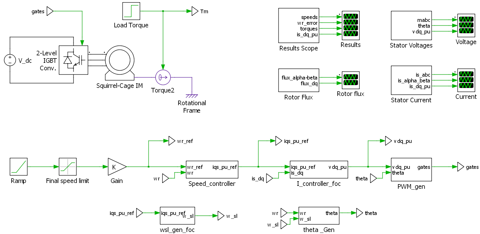
Figure 1. Indirect rotor flux oriented vector control
1 Initialization Parameters
%Motor parameters
- fbase=60;
- VLLBase=208;
- IpkBase=7.67;
- p=4;
- J=0.01;
- F=1e-3;
- Rr=0.6;
- Rs=1.5;
- Xlr=1.5;
- Xls=1.5;
- Xm=40;
%Current control parameters
- iqs_pu_limit=1.1;
- ids_pu_ref=0.5;
- PI_cur_kp=1;
- PI_cur_ki=10;
%DC source parameters
- VDC=350;
%Speed control parameters
- RampRate=2700;
- RampStartTime=1;
- InitialSlip=0;
- InitSpeedCommand=0;
- FinalUpperSpeedLimit=1800;
- FinalLowerSpeedLimit=0;
- TorqueStartTime=3;
- Tstart=0;
- Tfinal=6;
- PI_spd_kp=0.05;
- PI_spd_ki=0.05;
%Modulation parameters
- fs=2e3;
- vdq_pu_limit=1.15;
2 Objectives
In this lab you will use simulation to:
Investigate indirect rotor flux oriented vector control.
Investigate the design of PI control for an industrial drive.
3 Equipment
A computer with the PLECS Standalone installed.
You can download it from here. (https://www.plexim.com/download/standalone)
You should have been given a student code from the course instructor for a 1 year student license. Use this code in the PLECS License Manager to Request your Student license.
The ‘Lab 5.plecs’ model downloaded from the Lab 5 folder on eClass.
4 Experimental Procedure
Make sure to consider the Report Requirements before conducting the simulations so you understand what information you need to collect for your report. You may want to do all 5 parts first to familiarize yourself with the simulation results and note the parameters used for each and then go back to consider your simulation descriptions and to save your Waveform Comparisons using the procedure discussed below.
4.1 Waveform Comparison Procedure
You are asked to compare the results from:
part (1) with part (5)
part (3) comparing Kp and Ki set to 0.01, 0.1 and 1
parts (2), (3) and (4)
For instance, when comparing the plots from part (1) with part (5), run the simulation with the parameters for part (1). Double click the ‘Results Scope’ to open. In the toolbar at the top of the scopes screen you can click the following button to save the current waveforms to a set of’Traces’. You can rename this trace to something useful so you know which set of waveforms is saved under this name.

Hold current trace
Next to the saved trace you will see either a save trace button to save the most recent set of waveforms or a delete trace button to delete the associated waveforms. Both of the buttons shown below.

Save trace

Delete trace
Once simulation (1) is saved to a ‘Trace’, set the parameters for part (5) and run the simulation again. You should now have two sets of plots overlaid on each other for comparison. Add the new waveforms to a new trace if you wish to save them. You should now be able to export the waveforms to .pdf to include in your lab report, do not include a legend.
4.2 Simulations
4.2.1 Familiarization
Open the ‘Lab 5.plecs’ file in PLECS Standalone and begin to familiarize yourself with the model, variables and settings. The variable initialization parameters used in the simulation can be found by following the menu sequence. (Simulation - Simulation parameters… - Initialization)
Run the ‘Lab 5.plecs’ simulation as it is provided (Simulation – Start). Double click on the ‘Result Scope’ and note the following:
For the first second the speed control set point is set to 0 rpm and the controller is activated.
At 1 second the speed control set point is ramped to 1800 rpm.
- Parameters (RampRate=2700; RampStartTime=1; FinalUpperSpeedLimit=1800;)
At 3 seconds the load torque on the motor is switched from no-load to 6 Nm.
- Parameters (Tstart=0; Tfinal=6; TorqueStartTime=3;)
Open the other scope windows to view the other simulated waveforms to further familiarize yourself with indirect rotor flux oriented vector control.
Note: You will need to compare the ‘Results Scope’ of this simulation (1) to the final simulation (5) which has a better tuned speed control PI.
4.2.2 Default PI Speed Control Performance
Open the simulations initialization parameters by following the menu sequence (Simulation - Simulation parameters… - Initialization). Modify the appropriate parameters to accomplish the following:
For the speed set point to be 0 rpm for the entire simulation.
A step change in torque from 0 Nm to 6 Nm at 1 second.
Note the default Kp and Ki values for the speed control PI.
- Parameters (PI_spd_kp=0.05; PI_spd_ki=0.05;)
Run the simulation again with the new initialization parameters and observe the results.
Note: You will need to compare the ‘Results scope’ of this simulation (2) with the ‘Results scope’ from simulations (3) and (4).
4.2.3 Effect of Kp on Speed Control Performance (when Ki = Kp)
The purpose of this experiment is to obtain a suitable value for the proportional term Kp in the PI controlling the speed error. This is done by making Kp and Ki the same, and adjusting the two terms so that the peak speed error (maximum) during a transient is kept between an upper and lower bound.
Repeat simulation (2) with modified values of Kp and Ki for the speed control PI. Keep it so the Ki values are always equal to the kp values for this part (make Kp = Ki). Try values of 0.01, 0.1 and 1 and determine which values give you a peak (maximum) speed error ‘wr_error’ that lies between 6 and 7 electrical radians/second. Use these new values for Kp and Ki at the beginning of simulation (4).
Note: You will need to compare the ‘Results scope’ with the error between 6 and 7 electrical radians/second with the ‘Results scope’ from simulations (2) and (4).
4.2.4 Impact of Ki on Speed Control Performance
Having got a suitable value for Kp, the purpose of this experiment is to obtain a suitable value for the integral term Ki in the PI controlling the speed error. This is done by keeping the Kp value obtained from part (3) and adjusting Ki so that the speed error 1 sec after the torque transient is kept between an upper and lower bound.
Repeat simulation (3) with a modified value of Ki for the speed control PI. This time continue modifying Ki until you obtain a speed error ‘wr_error’ at 2 seconds that lies between 0.3 and 0.4 radians/second. Use these new values for Kp and Ki at the beginning of simulation (5).
Note: You will need to compare the ‘Results scope’ with the error between 0.3 and 0.4 electrical radians/second with the ‘Results scope’ from simulations (2) and (3).
4.2.5 Observe Improved Speed Control Performance with New Kp and Ki Values.
With the new values on Kp and Ki for the speed control PI simulate the original speed ramp and torque step transients used in simulation (1).
Using “Waveform Comparison Procedure” described above, compare the waveform plots from the Results scope in parts (1) and (5).
Note: You will need to compare the ‘Results Scope’ of this simulation (5) to the first simulation (1) which has the original values for the speed control PI.
5 Report Requirements
Include the waveform comparison plots from the ‘Results Scope’ that compares the waveform results from simulations (1) and (5).
Describe the operation of the vector controlled drive from parts (1) and (5). Think in terms of the system operation vs. time, e.g.:
t = 0 to 1 seconds: the system is initializing, explain what is happening and how.
t = 1 second: the commanded speed increases, explain how the system responds.
t = 3 second: there is a step change in torque, explain how the system responds.
Include the waveform comparison plots from the ‘Results Scope’ that compares the waveform results from simulations (2), (3) and (4).
Describe the operation of the vector controlled drive from parts (2), (3), (4). Describe what you have changed from one simulation to the next; describe and explain the impact of your changes. Think in terms of the system operation vs. time, e.g.:
t = 0 to 1 seconds: the system is initializing, explain what is happening and how.
t = 1 second: there is a step change in torque, explain how the system responds.
Include the waveform comparison plots from the ‘Results Scope’ that compares the waveform results from simulation (3) when the Kp and Ki values are set at 0.01, 0.1 and 1.