Lab 4 - Open-loop Drive Control
ECE432 - Variable Speed Drives
Electrical and Computer Engineering - University of Alberta
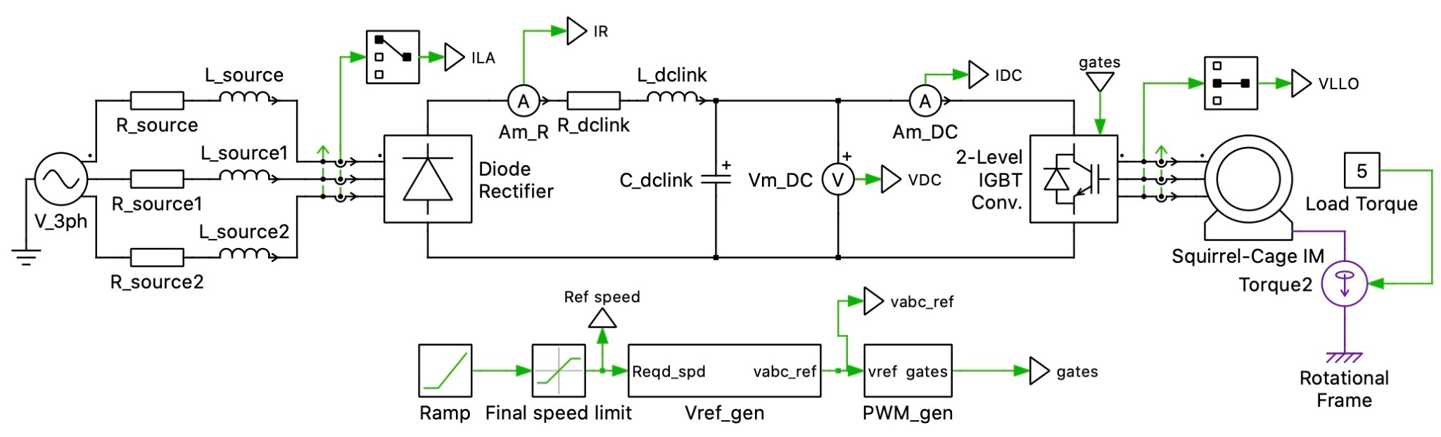
Figure 1. PLECS Schematic - Open loop drive control
1 Initialization Parameters
%Motor parameters
fbase=60; fbrake=15; VLLBase=240; p=4; J=0.01; F=1e-3; Rr=0.6; Rs=1.5; Xlr=1.5; Xls=1.5; Xm=70;
%DC-Link parameters
DCCap=1e-3; DCL=10e-3; DCR=1e-5;
%Control parameters
RampRate=0; RampStartTime=0; InitialSlip=0; InitSpeedCommand=1800; FinalUpperSpeedLimit=1800; FinalLowerSpeedLimit=0; fs=2e3;
%AC source parameters
fsupply=60; VLLS=240; Rsource=0.02; Lsource=100e-6;
2 Objectives
In this lab you will use simulation to:
see the effects of inductance and capacitance on drive performance.
see the effects of switching frequency on motor currents.
see the dynamic effects of drive-motor interaction.
3 Equipment
A computer with the PLECS Standalone installed.
You can download it from here: (https://www.plexim.com/download/standalone)
Use the required student code that is available on eClass to obtain a 1 year student license. Follow the instructions to obtain a license here: (https://www.plexim.com/store/students)
The required PLECS models downloaded from eClass.
4 Experimental Procedure
Download the PLECS model files from eclass under lab 4.
Open the PLECS simulation file Lab_4a.plecs for the first experiment and become familiar with the variables, settings and operation of the simulation. The drive parameters used in the simulation can be found by following the menu sequence: (Simulation -> Simulation parameters -> Initialization). At this time you can select the dc link inductor to be 50 µH, and the ac supply inductance to be 100 µH, dc capacitor to be 200 µH.
4.1 Effect of dc capacitance, ac and dc inductance values.
In the first part of the lab you will investigate the impact of the ac/dc inductors, dc capacitance voltage, input current and its THD. You are required to repeat a simulation of the machine operating in steady state at 60Hz open loop with a 5 Nm load. For each simulation you will need to record data from the scope outputs of the simulation (once steady state has been reached) and analyze this data.
4.1.1 PLECS Setup Procedure
Set the simulation parameters (simulation submenu) to have a simulation start time of 0 and a stop time of 0.41667 sec.
After each simulation, double click the scope labeled “rectifier scope” to observe the waveforms. Then double click the time scale underneath the bottom waveform. Set the time scale “Lower limit” value to 0.4 and the “Upper Limit” value to 0.41667 secs. This allows you to observe the waveforms over one complete ac supply cycle.
Under the scope “view” menu, select “fourier spectrum” and set the base frequency to 60 Hz. This must be done before the next step where you select “waveform analysis”.
Under the scope “view” menu you can select “waveform analysis” which has the measurement parameters: delta, min, max, absMax, mean, RMS and THD. This will give you these parameters for each waveform viewed in the scope over the simulation time period chosen (a data window will appear below the waveforms). Useful parameters to select for this part of the lab are: min, max, mean, RMS and THD. Note that the THD is not in % and should be multiplied by 100.
Save the waveforms using the scope menu sequence (File -> Export -> as PDF). Choose “line style” “black and white”. Choose a file name to identify the data being saved.
For each of the 3 simulation cases described below you should use the Plecs “waveform analysis” menu in the scope labeled “rectifier scope” to obtain:
line supply current RMS and THD (=ipha)
DC and peak-peak ripple of capacitor voltage (= dc link voltage Vdc).
DC and peak-peak ripple of the dc inductor current (= iLdc in the scope waveforms).
- After obtaining each set of data, save your waveforms to a pdf file. These plots should be included in your final report.
4.1.2 Simulation Cases (1, 2 and 3)
4.1.2.1 Part 1 - Negligible Supply and DC-link Inductance (Ldc = 50µH, Lac = 100µH)
Simulate the operation of the system with the following DC link Capacitance values: 200 µF, 500 µF and 1000 µF.
4.1.2.2 Part 2 - Negligible DC-link Inductance, added Supply Inductance
Calculate the base reactance for a 1.5kVA, 208V system and the value of inductance that corresponds to 1, 2, 5, 10 % relative to the base inductance (e.g. 1% = 0.01 p.u.). Set the supply inductance to each value and simulate using Cdc = 1000 µF. In your results table quote the inductance used in mH.
4.1.2.3 Part 3 - Added DC-link Inductance and a limited ac supply Inductance
With the ac supply inductance set to 100 µH. Choose DC-link inductances of 1, 2.5, 5, 10 mH. Set the dc inductance to each value and simulate using Cdc = 1000 µF.
4.1.3 Report Requirements (1, 2 and 3)
For each simulation undertaken, your report should tabulate the supply current THD & RMS values, average and peak-peak ripple of the dc link current (inductor current), the DC and peak-peak ripple of the capacitor voltage. Include the plots that you obtained. For parts 1 to 3, explain how, and why, the choice of component size affects:
THD & RMS of the supply current
average & pk-pk ripple of the dc link inductor current
average & pk-pk ripple of the dc capacitor voltage
4.2 Impact of Switching Frequency
4.2.1 PLECS Setup Procedure
Use the PLECS simulation file Lab_4b.plecs.
Open the Initialization parameters for the simulation by navigating to (Simulation -> Simulation parameters -> Initialization) and ensure that the following things are set:
ac inductance = 100 µH
dc inductance = 10 mH
dc capacitance = 1 mH.
switching frequency = 2kHz
Set the simulation parameters to have a simulation start time of 0 and a stop time of 0.41667 sec.
After the simulation double click the scope “motor scope” to observe the waveforms. Then double click the time scale underneath the bottom waveform. Set the time scale “Lower limit” value to 0.4 and the “Upper limit” value to 0.41667 secs. This allows you to observe the waveforms over one complete ac supply cycle.
Under the scope “View” menu, select “Fourier spectrum” and set the base frequency to 60 Hz. This must be done before the next step where you select “waveform analysis”.
Under the scope “View” menu you can hover over “Analysis” which has the following measurement parameters checkboxes: delta, min, max, absMax, mean, RMS and THD. Each checkbox will give you the corresponding parameters (a data window will appear below the waveforms) for each of the waveforms viewed in the scope over the simulation time period chosen. The useful parameters to select for this part of the lab are: RMS and THD. Note that the THD is not in % and should be multiplied by 100.
4.2.2 Simulation Case (4)
4.2.2.1 Part 4 - Motor RMS Current and THD
Change the stop time of the simulation to 4.5 seconds and run the simulation again.
Set the “motor scopes” scales to the following.
Time to 0.4 second “Lower limit” and 0.45 second “Upper limit.
Motor Speed scale 1700 to 1800 rpm.
Motor Torque scale 0 to 7 Nm.
Stator Current scale to -6 to 6 A.
Record the Mean, RMS and THD for all the waveforms.
Save the waveforms using the scope menu sequence (File - Export - as PDF). Choose a file name to identify the data being saved and the circuit parameters being used. Make sure you use the black and white option for the waveforms.
Repeat this simulation with the switching frequency of the inverter increased to 5 kHz and record the same information again.
4.2.3 Report Requirements (4)
Your report should include the required plots captured from PLECS as well as the measurements you obtained from them. Using these results also answer the following questions.
Why the stator current THD is smaller than the voltage THD.
Why the stator current RMS and THD changes with frequency but the line voltage does not.
Using the steady state motor speed and knowing the motor's synchronous speed determine the motor mechanical slip frequency in both rpm and the machine's electrical slip frequency in rad/sec.
Account for the average motor torque value. Account for why the inverter switching frequency has an effect on the torque high frequency ripple.
4.3 Dynamic Simulations
4.3.1 (5) Simulation Case (5)
4.3.1.1 Part 5 - Line-Start
Use PLECS to open and simulate the provided simulation file Lab_4c.plecs.
Set the simulation time to 0.4 secs.
Run the simulation and set the motor speed scale to 0 to 2000 rpm. The automatic scales used for the torque and motor current should be OK. Save the waveforms (stator current, motor torque, motor speed in rpm) to a pdf file. Make sure that you use the black and white option for the waveforms.
From the plots determine the following:
Peak-peak of the motor current around 0.02 sec and at 0.4 secs.
Motor torque at approx 0.11 secs and then again at 0.4 secs.
The approx time it takes for the motor to accelerate up to full speed, and its value at 0.4 secs.
4.3.2 Report Requirements (5)
Your report should include the required 3 plots captured from PLECS as well as the measurements you obtained from them. Using these results also answer the following question.
Use the measured peak-peak motor current values of the stator to approximate the maximum rms current of the motor during start up as well as when it reaches steady state. Calculate the ratio between these two values and explain its significance?
Account for the motor torque value obtained at 0.4 secs. Account for the relative magnitude of the motor torque measured at 0.11 secs compared to that measured at 0.4 secs.
Account for the motor speed measured at 0.4 secs by quoting the motor synchronous speed and the slip frequency in rpm.
4.3.3 Simulation Case (6)
4.3.3.1 Part 6 - Ramp-Start
Use PLECS to open and simulate the provided simulation file Lab_4d.plecs. Set the motor speed to ramp up from 0 rpm to 1800 rpm over a period of 2 seconds. Set the following parameters in the initialize menu:
RampRate=1800;
InitialSlip=1;
InitSpeedCommand=0;
Total simulation time of 1.5 seconds.
After simulating, save the waveform plots for torque, speed and current to a pdf file. Make sure you use the black and white option for the waveforms.
As the machine is still accelerating, determine both the motor current and motor torque around the 0.6 secs mark. Make sure to neglect the initial transient which occurs upto approximately 0.5 secs. Then compare these values by measuring them again after the machine reaches its full speed.
Determine the maximum peak current of the machine during its ramp-start.
4.3.4 Report Requirements (6)
Your report should include the required 3 plots captured from PLECS as well as the measurements you obtained from them. Using these results also answer the following question.
- Explain in your own words why the motor current and torque during acceleration is larger than that once the machine reaches full speed.
4.3.5 Simulation Case (7)
4.3.5.1 Part 7 - Torque Variation
Use PLECS to open and simulate the provided simulation file Lab_4e.plecs.
The circuit is set up with the initial slip value to 0 and commanded speed to 1800rpm.
The load torque is set to change from 5 Nm t = 0 to 1 sec, 10 Nm t = 1 to 2 secs, and 0 N-m t = 2 to 3 secs.
The simulation duration is set to 3 seconds.
After simulating, set the current scale to (-20 to 20 A), the torque scale to (-5 to 20 Nm), the speed scale to (1700 to 1850 rpm) and save the three plots to a pdf file. Make sure you use the black and white option for the waveforms.
For the time periods 0 to 1 sec, 1 to 2 secs and 2 to 3 seconds from each of the plots, determine the values for the motor rms current, the mean speed in rpm, and mean torque in Nm.
4.3.6 Report Requirements (7)
Your report should include the required 3 plots captured from PLECS as well as the measurements you obtained from them. Using these results also answer the following question.
- Are the torque, current and speed waveforms what you would expect? Explain in your own words what is happening to the machine during 3 seconds of the simulation.